23 Hierarchical data

23.1 Introduction

In this chapter, you’ll learn the art of data rectangling: taking data that is fundamentally hierarchical, or tree-like, and converting it into a rectangular data frame made up of rows and columns. This is important because hierarchical data is surprisingly common, especially when working with data that comes from the web.
在本章中，你将学习数据矩形化 (rectangling) 的艺术：将本质上是分层的或树状的数据，转换为由行和列组成的矩形数据框。这一点很重要，因为分层数据出人意料地常见，尤其是在处理来自网络的数据时。

To learn about rectangling, you’ll need to first learn about lists, the data structure that makes hierarchical data possible. Then you’ll learn about two crucial tidyr functions: tidyr::unnest_longer() and tidyr::unnest_wider(). We’ll then show you a few case studies, applying these simple functions again and again to solve real problems. We’ll finish off by talking about JSON, the most frequent source of hierarchical datasets and a common format for data exchange on the web.
要学习矩形化，你需要先了解列表，这种数据结构使分层数据成为可能。然后你将学习两个关键的 tidyr 函数：tidyr::unnest_longer() 和 tidyr::unnest_wider()。接着，我们将通过一些案例研究，反复应用这些简单的函数来解决实际问题。最后，我们将讨论 JSON，它是分层数据集最常见的来源，也是网络上数据交换的常用格式。

23.1.1 Prerequisites

In this chapter, we’ll use many functions from tidyr, a core member of the tidyverse. We’ll also use repurrrsive to provide some interesting datasets for rectangling practice, and we’ll finish by using jsonlite to read JSON files into R lists.
在本章中，我们将使用许多来自 tidyr 的函数，它是 tidyverse 的核心成员。我们还将使用 repurrrsive 包来提供一些有趣的数据集，用于矩形化练习，最后我们将使用 jsonlite 包将 JSON 文件读入 R 列表。

library(tidyverse)
library(repurrrsive)
library(jsonlite)

23.2 Lists

So far you’ve worked with data frames that contain simple vectors like integers, numbers, characters, date-times, and factors. These vectors are simple because they’re homogeneous: every element is of the same data type. If you want to store elements of different types in the same vector, you’ll need a list, which you create with list():
到目前为止，你所使用的数据框包含的是简单的向量，如整数、数字、字符、日期时间和因子。这些向量之所以简单，是因为它们是同质的：每个元素都属于相同的数据类型。如果你想在同一个向量中存储不同类型的元素，你就需要一个列表 (list)，你可以用 list() 来创建它：

x1 <- list(1:4, "a", TRUE)
x1
#> [[1]]
#> [1] 1 2 3 4
#> 
#> [[2]]
#> [1] "a"
#> 
#> [[3]]
#> [1] TRUE

It’s often convenient to name the components, or children, of a list, which you can do in the same way as naming the columns of a tibble:
为列表的组件（或称子元素 (children)）命名通常很方便，你可以像命名 tibble 的列一样来做：

x2 <- list(a = 1:2, b = 1:3, c = 1:4)
x2
#> $a
#> [1] 1 2
#> 
#> $b
#> [1] 1 2 3
#> 
#> $c
#> [1] 1 2 3 4

Even for these very simple lists, printing takes up quite a lot of space. A useful alternative is str(), which generates a compact display of the structure, de-emphasizing the contents:
即使是这些非常简单的列表，打印出来也会占用相当大的空间。一个有用的替代方法是 str()，它会生成一个紧凑的结构 (structure) 显示，并淡化其内容：

str(x1)
#> List of 3
#>  $ : int [1:4] 1 2 3 4
#>  $ : chr "a"
#>  $ : logi TRUE
str(x2)
#> List of 3
#>  $ a: int [1:2] 1 2
#>  $ b: int [1:3] 1 2 3
#>  $ c: int [1:4] 1 2 3 4

As you can see, str() displays each child of the list on its own line. It displays the name, if present, then an abbreviation of the type, then the first few values.
如你所见，str() 将列表的每个子元素显示在单独的一行上。它会显示名称（如果存在），然后是类型的缩写，最后是前几个值。

23.2.1 Hierarchy

Lists can contain any type of object, including other lists. This makes them suitable for representing hierarchical (tree-like) structures:
列表可以包含任何类型的对象，包括其他列表。这使得它们非常适合表示分层（树状）结构：

x3 <- list(list(1, 2), list(3, 4))
str(x3)
#> List of 2
#>  $ :List of 2
#>   ..$ : num 1
#>   ..$ : num 2
#>  $ :List of 2
#>   ..$ : num 3
#>   ..$ : num 4

This is notably different to c(), which generates a flat vector:
这与 c() 函数显著不同，c() 函数会生成一个扁平的向量：

c(c(1, 2), c(3, 4))
#> [1] 1 2 3 4

x4 <- c(list(1, 2), list(3, 4))
str(x4)
#> List of 4
#>  $ : num 1
#>  $ : num 2
#>  $ : num 3
#>  $ : num 4

As lists get more complex, str() gets more useful, as it lets you see the hierarchy at a glance:
随着列表变得越来越复杂，str() 的用处也越来越大，因为它能让你一目了然地看到层级结构：

x5 <- list(1, list(2, list(3, list(4, list(5)))))
str(x5)
#> List of 2
#>  $ : num 1
#>  $ :List of 2
#>   ..$ : num 2
#>   ..$ :List of 2
#>   .. ..$ : num 3
#>   .. ..$ :List of 2
#>   .. .. ..$ : num 4
#>   .. .. ..$ :List of 1
#>   .. .. .. ..$ : num 5

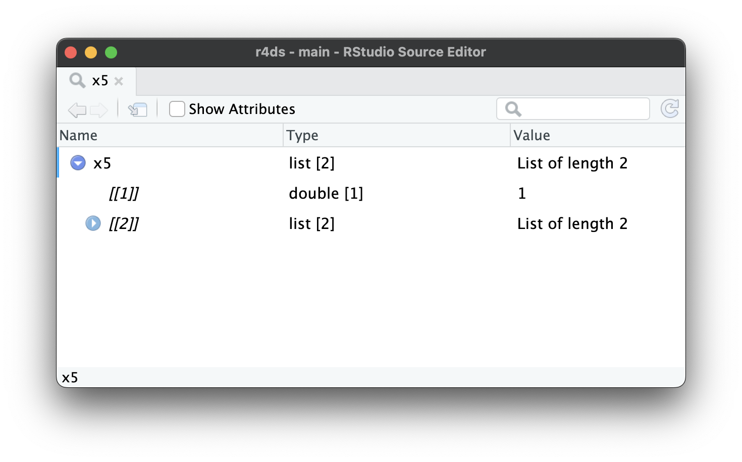
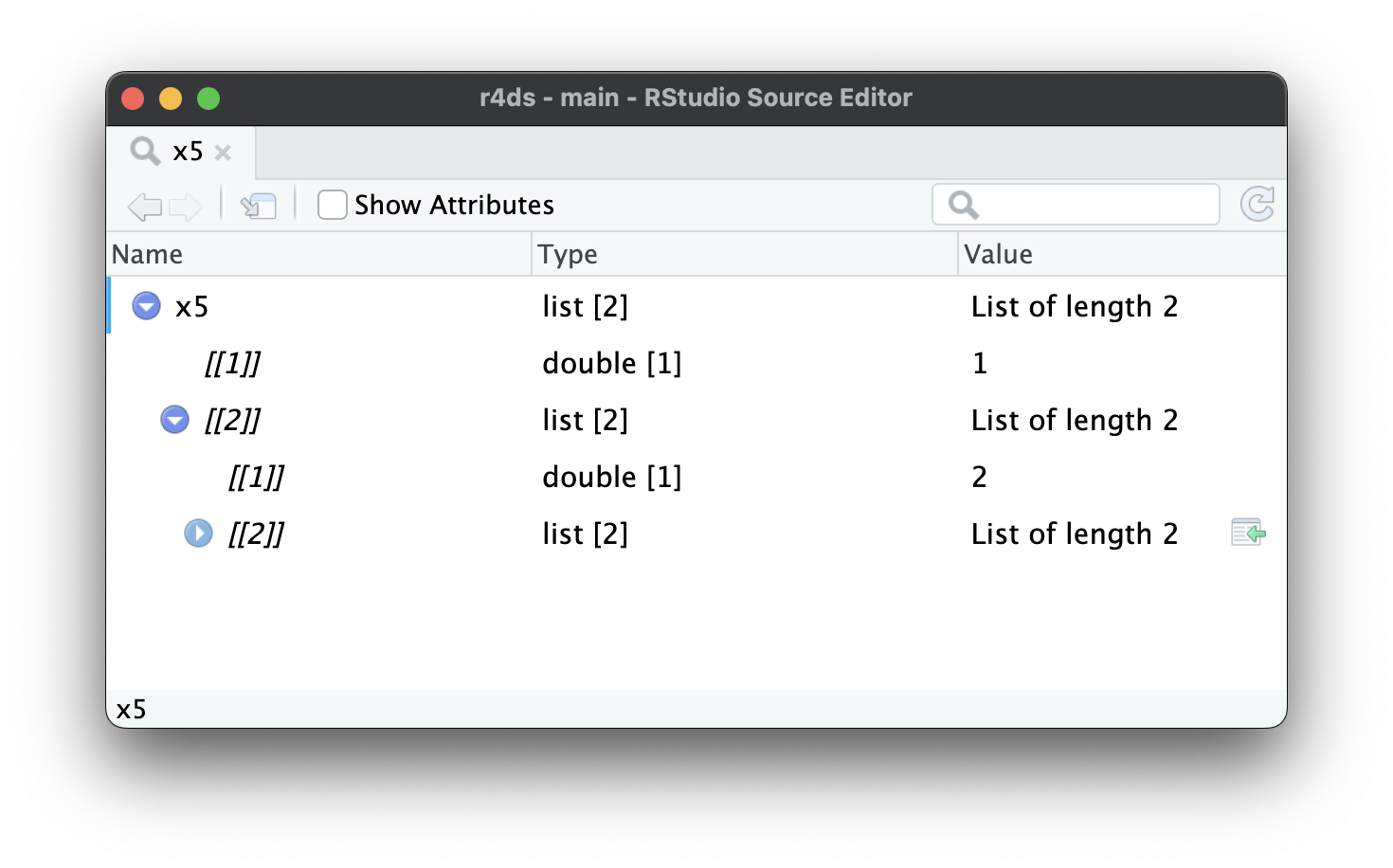
As lists get even larger and more complex, str() eventually starts to fail, and you’ll need to switch to View()¹. Figure 23.1 shows the result of calling View(x5). The viewer starts by showing just the top level of the list, but you can interactively expand any of the components to see more, as in Figure 23.2. RStudio will also show you the code you need to access that element, as in Figure 23.3. We’ll come back to how this code works in Section 27.3.
当列表变得更大、更复杂时，str() 最终会变得力不从心，这时你就需要切换到 View() ¹。Figure 23.1 展示了调用 View(x5) 的结果。查看器开始时只显示列表的顶层，但你可以交互式地展开任何组件以查看更多内容，如 Figure 23.2 所示。RStudio 还会向你显示访问该元素所需代码，如 Figure 23.3 所示。我们将在 Section 27.3 回顾这段代码是如何工作的。

A screenshot of RStudio showing the list-viewer. It shows the two children of x5: the first child is a double vector and the second child is a list. A rightward facing triable indicates that the second child itself has children but you can't see them. — Figure 23.1: The RStudio view lets you interactively explore a complex list. The viewer opens showing only the top level of the list.

Another screenshot of the list-viewer having expand the second child of x5. It also has two children, a double vector and another list. — Figure 23.2: Clicking on the rightward facing triangle expands that component of the list so that you can also see its children.

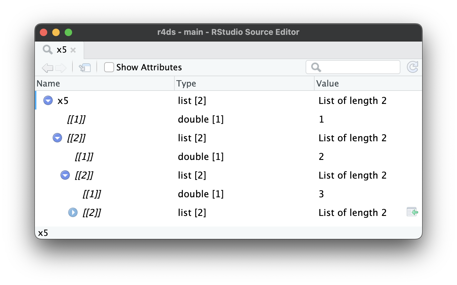
Another screenshot, having expanded the grandchild of x5 to see its two children, again a double vector and a list. — Figure 23.3: You can repeat this operation as many times as needed to get to the data you’re interested in. Note the bottom-left corner: if you click an element of the list, RStudio will give you the subsetting code needed to access it, in this case `x5[[2]][[2]][[2]]`.

23.2.2 List-columns

Lists can also live inside a tibble, where we call them list-columns. List-columns are useful because they allow you to place objects in a tibble that wouldn’t usually belong in there. In particular, list-columns are used a lot in the tidymodels ecosystem, because they allow you to store things like model outputs or resamples in a data frame.
列表也可以存在于 tibble 中，我们称之为列表列 (list-columns)。列表列很有用，因为它们允许你将通常不属于 tibble 的对象放入其中。特别地，列表列在 tidymodels 生态系统中被大量使用，因为它们允许你将模型输出或重采样等内容存储在数据框中。

Here’s a simple example of a list-column:
下面是列表列的一个简单示例：

df <- tibble(
  x = 1:2, 
  y = c("a", "b"),
  z = list(list(1, 2), list(3, 4, 5))
)
df
#> # A tibble: 2 × 3
#>       x y     z         
#>   <int> <chr> <list>    
#> 1     1 a     <list [2]>
#> 2     2 b     <list [3]>

There’s nothing special about lists in a tibble; they behave like any other column:
tibble 中的列表没有什么特别之处；它们的行为与任何其他列一样：

df |> 
  filter(x == 1)
#> # A tibble: 1 × 3
#>       x y     z         
#>   <int> <chr> <list>    
#> 1     1 a     <list [2]>

Computing with list-columns is harder, but that’s because computing with lists is harder in general; we’ll come back to that in Chapter 26. In this chapter, we’ll focus on unnesting list-columns out into regular variables so you can use your existing tools on them.
使用列表列进行计算更加困难，但这是因为通常情况下使用列表进行计算就更难；我们将在 Chapter 26 回到这个问题。在本章中，我们将专注于将列表列“展开” (unnesting) 为常规变量，以便你可以使用现有的工具来处理它们。

The default print method just displays a rough summary of the contents. The list column could be arbitrarily complex, so there’s no good way to print it. If you want to see it, you’ll need to pull out just the one list-column and apply one of the techniques that you’ve learned above, like df |> pull(z) |> str() or df |> pull(z) |> View().
默认的打印方法只显示了内容的粗略摘要。列表列可能任意复杂，所以没有很好的方法来打印它。如果你想查看它，你需要单独抽取出那个列表列，并应用你上面学到的技术之一，比如 df |> pull(z) |> str() 或 df |> pull(z) |> View()。

Base R

It’s possible to put a list in a column of a data.frame, but it’s a lot fiddlier because data.frame() treats a list as a list of columns:
可以在 data.frame 的一列中放入一个列表，但这要麻烦得多，因为 data.frame() 将列表视为列的列表：

data.frame(x = list(1:3, 3:5))
#>   x.1.3 x.3.5
#> 1     1     3
#> 2     2     4
#> 3     3     5

You can force data.frame() to treat a list as a list of rows by wrapping it in list I(), but the result doesn’t print particularly well:
你可以通过将列表包装在 I() 中来强制 data.frame() 将其视为行的列表，但结果打印得不是特别好：

data.frame(
  x = I(list(1:2, 3:5)), 
  y = c("1, 2", "3, 4, 5")
)
#>         x       y
#> 1    1, 2    1, 2
#> 2 3, 4, 5 3, 4, 5

It’s easier to use list-columns with tibbles because tibble() treats lists like vectors and the print method has been designed with lists in mind.
使用 tibble 来处理列表列更容易，因为 tibble() 将列表视为向量，并且其打印方法是为列表而专门设计的。

23.3 Unnesting

Now that you’ve learned the basics of lists and list-columns, let’s explore how you can turn them back into regular rows and columns. Here we’ll use very simple sample data so you can get the basic idea; in the next section we’ll switch to real data.
既然你已经了解了列表和列表列的基础知识，让我们来探讨如何将它们转换回常规的行和列。这里我们将使用非常简单的示例数据，以便你掌握基本概念；在下一节中，我们将转向真实数据。

List-columns tend to come in two basic forms: named and unnamed. When the children are named, they tend to have the same names in every row. For example, in df1, every element of list-column y has two elements named a and b. Named list-columns naturally unnest into columns: each named element becomes a new named column.
列表列通常有两种基本形式：命名的和未命名的。当子元素是命名的 (named) 时，它们在每一行中往往具有相同的名称。例如，在 df1 中，列表列 y 的每个元素都有两个名为 a 和 b 的元素。命名的列表列很自然地可以展开为列：每个命名元素都会成为一个新的命名列。

df1 <- tribble(
  ~x, ~y,
  1, list(a = 11, b = 12),
  2, list(a = 21, b = 22),
  3, list(a = 31, b = 32),
)

When the children are unnamed, the number of elements tends to vary from row-to-row. For example, in df2, the elements of list-column y are unnamed and vary in length from one to three. Unnamed list-columns naturally unnest into rows: you’ll get one row for each child.
当子元素是未命名的 (unnamed) 时，元素的数量往往因行而异。例如，在 df2 中，列表列 y 的元素是未命名的，并且长度从一到三不等。未命名的列表列很自然地可以展开为行：每个子元素都会生成新的一行。

df2 <- tribble(
  ~x, ~y,
  1, list(11, 12, 13),
  2, list(21),
  3, list(31, 32),
)

tidyr provides two functions for these two cases: unnest_wider() and unnest_longer(). The following sections explain how they work.
tidyr 为这两种情况提供了两个函数：unnest_wider() 和 unnest_longer()。以下各节将解释它们的工作原理。

23.3.1 `unnest_wider()`

When each row has the same number of elements with the same names, like df1, it’s natural to put each component into its own column with unnest_wider():
当每一行都有相同数量且名称相同的元素时，就像 df1 一样，很自然地可以使用 unnest_wider() 将每个组件放入各自的列中：

df1 |> 
  unnest_wider(y)
#> # A tibble: 3 × 3
#>       x     a     b
#>   <dbl> <dbl> <dbl>
#> 1     1    11    12
#> 2     2    21    22
#> 3     3    31    32

By default, the names of the new columns come exclusively from the names of the list elements, but you can use the names_sep argument to request that they combine the column name and the element name. This is useful for disambiguating repeated names.
默认情况下，新列的名称完全来自列表元素的名称，但你可以使用 names_sep 参数来要求它们合并列名和元素名。这对于消除重复名称的歧义很有用。

df1 |> 
  unnest_wider(y, names_sep = "_")
#> # A tibble: 3 × 3
#>       x   y_a   y_b
#>   <dbl> <dbl> <dbl>
#> 1     1    11    12
#> 2     2    21    22
#> 3     3    31    32

23.3.2 `unnest_longer()`

When each row contains an unnamed list, it’s most natural to put each element into its own row with unnest_longer():
当每一行都包含一个未命名的列表时，最自然的做法是使用 unnest_longer() 将每个元素放入其自己的行中：

df2 |> 
  unnest_longer(y)
#> # A tibble: 6 × 2
#>       x     y
#>   <dbl> <dbl>
#> 1     1    11
#> 2     1    12
#> 3     1    13
#> 4     2    21
#> 5     3    31
#> 6     3    32

Note how x is duplicated for each element inside of y: we get one row of output for each element inside the list-column. But what happens if one of the elements is empty, as in the following example?
注意 x 是如何为 y 内的每个元素复制的：对于列表列中的每个元素，我们都会得到一行输出。但是，如果其中一个元素为空，如下面的例子所示，会发生什么呢？

df6 <- tribble(
  ~x, ~y,
  "a", list(1, 2),
  "b", list(3),
  "c", list()
)
df6 |> unnest_longer(y)
#> # A tibble: 3 × 2
#>   x         y
#>   <chr> <dbl>
#> 1 a         1
#> 2 a         2
#> 3 b         3

We get zero rows in the output, so the row effectively disappears. If you want to preserve that row, adding NA in y, set keep_empty = TRUE.
我们在输出中得到零行，因此该行实际上消失了。如果你想保留那一行，并在 y 中添加 NA，请设置 keep_empty = TRUE。

23.3.3 Inconsistent types

What happens if you unnest a list-column that contains different types of vector? For example, take the following dataset where the list-column y contains two numbers, a character, and a logical, which can’t normally be mixed in a single column.
如果你展开一个包含不同类型向量的列表列，会发生什么？例如，看下面这个数据集，其中列表列 y 包含两个数字、一个字符和一个逻辑值，这些通常不能在单个列中混合。

df4 <- tribble(
  ~x, ~y,
  "a", list(1),
  "b", list("a", TRUE, 5)
)

unnest_longer() always keeps the set of columns unchanged, while changing the number of rows. So what happens? How does unnest_longer() produce five rows while keeping everything in y?
unnest_longer() 总是保持列集合不变，同时改变行的数量。那么会发生什么呢？unnest_longer() 是如何在保持 y 中所有内容的同时生成五行的呢？

df4 |> 
  unnest_longer(y)
#> # A tibble: 4 × 2
#>   x     y        
#>   <chr> <list>   
#> 1 a     <dbl [1]>
#> 2 b     <chr [1]>
#> 3 b     <lgl [1]>
#> 4 b     <dbl [1]>

As you can see, the output contains a list-column, but every element of the list-column contains a single element. Because unnest_longer() can’t find a common type of vector, it keeps the original types in a list-column. You might wonder if this breaks the commandment that every element of a column must be the same type. It doesn’t: every element is a list, even though the contents are of different types.
正如你所见，输出包含一个列表列，但该列表列的每个元素都只包含一个单一元素。因为 unnest_longer() 找不到一个通用的向量类型，所以它将原始类型保留在一个列表列中。你可能会好奇这是否违反了“列的每个元素必须是相同类型”的规定。答案是否定的：每个元素都是一个列表，尽管其内容是不同类型的。

Dealing with inconsistent types is challenging and the details depend on the precise nature of the problem and your goals, but you’ll most likely need tools from Chapter 26.
处理不一致的类型是具有挑战性的，具体细节取决于问题的确切性质和你的目标，但你很可能需要来自 Chapter 26 的工具。

23.3.4 Other functions

tidyr has a few other useful rectangling functions that we’re not going to cover in this book:
tidyr 还有一些其他有用的矩形化函数，我们在这本书中不会涉及：

unnest_auto() automatically picks between unnest_longer() and unnest_wider() based on the structure of the list-column. It’s great for rapid exploration, but ultimately it’s a bad idea because it doesn’t force you to understand how your data is structured, and makes your code harder to understand.
unnest_auto() 会根据列表列的结构自动在 unnest_longer() 和 unnest_wider() 之间进行选择。它非常适合快速探索，但最终来说，这是一个坏主意，因为它不会迫使你去理解你的数据结构，并使你的代码更难理解。
unnest() expands both rows and columns. It’s useful when you have a list-column that contains a 2d structure like a data frame, which you don’t see in this book, but you might encounter if you use the tidymodels ecosystem.
unnest() 会同时扩展行和列。当你的列表列包含像数据框这样的二维结构时，它很有用，这在本书中你不会看到，但如果你使用 tidymodels 生态系统，你可能会遇到。

These functions are good to know about as you might encounter them when reading other people’s code or tackling rarer rectangling challenges yourself.
了解这些函数是很有好处的，因为在阅读他人的代码或自己处理更罕见的矩形化挑战时，你可能会遇到它们。

23.3.5 Exercises

What happens when you use unnest_wider() with unnamed list-columns like df2? What argument is now necessary? What happens to missing values?
What happens when you use unnest_longer() with named list-columns like df1? What additional information do you get in the output? How can you suppress that extra detail?
From time-to-time you encounter data frames with multiple list-columns with aligned values. For example, in the following data frame, the values of y and z are aligned (i.e. y and z will always have the same length within a row, and the first value of y corresponds to the first value of z). What happens if you apply two unnest_longer() calls to this data frame? How can you preserve the relationship between x and y? (Hint: carefully read the docs).
```
df4 <- tribble(
  ~x, ~y, ~z,
  "a", list("y-a-1", "y-a-2"), list("z-a-1", "z-a-2"),
  "b", list("y-b-1", "y-b-2", "y-b-3"), list("z-b-1", "z-b-2", "z-b-3")
)
```

23.4 Case studies

The main difference between the simple examples we used above and real data is that real data typically contains multiple levels of nesting that require multiple calls to unnest_longer() and/or unnest_wider(). To show that in action, this section works through three real rectangling challenges using datasets from the repurrrsive package.
我们上面使用的简单示例与真实数据之间的主要区别在于，真实数据通常包含多个嵌套层级，需要多次调用 unnest_longer() 和/或 unnest_wider()。为了实际展示这一点，本节将使用来自 repurrrsive 包的数据集，通过三个真实的矩形化挑战来进行讲解。

23.4.1 Very wide data

We’ll start with gh_repos. This is a list that contains data about a collection of GitHub repositories retrieved using the GitHub API. It’s a very deeply nested list so it’s difficult to show the structure in this book; we recommend exploring a little on your own with View(gh_repos) before we continue.
我们从 gh_repos 开始。这是一个列表，其中包含通过 GitHub API 检索到的关于一组 GitHub 仓库的数据。这是一个非常深层嵌套的列表，因此很难在本书中展示其结构；我们建议在继续之前，你可以自己用 View(gh_repos) 稍作探索。

gh_repos is a list, but our tools work with list-columns, so we’ll begin by putting it into a tibble. We call this column json for reasons we’ll get to later.
gh_repos 是一个列表，但我们的工具是针对列表列工作的，所以我们首先要把它放进一个 tibble 中。我们将这一列命名为 json，原因稍后会解释。

repos <- tibble(json = gh_repos)
repos
#> # A tibble: 6 × 1
#>   json       
#>   <list>     
#> 1 <list [30]>
#> 2 <list [30]>
#> 3 <list [30]>
#> 4 <list [26]>
#> 5 <list [30]>
#> 6 <list [30]>

This tibble contains 6 rows, one row for each child of gh_repos. Each row contains an unnamed list with either 26 or 30 rows. Since these are unnamed, we’ll start with unnest_longer() to put each child in its own row:
这个 tibble 包含 6 行，gh_repos 的每个子元素占一行。每一行都包含一个未命名的列表，该列表有 26 或 30 行。由于这些列表是未命名的，我们先使用 unnest_longer() 将每个子元素放到单独的行中：

repos |> 
  unnest_longer(json)
#> # A tibble: 176 × 1
#>   json             
#>   <list>           
#> 1 <named list [68]>
#> 2 <named list [68]>
#> 3 <named list [68]>
#> 4 <named list [68]>
#> 5 <named list [68]>
#> 6 <named list [68]>
#> # ℹ 170 more rows

At first glance, it might seem like we haven’t improved the situation: while we have more rows (176 instead of 6) each element of json is still a list. However, there’s an important difference: now each element is a named list so we can use unnest_wider() to put each element into its own column:
乍一看，情况似乎并没有改善：虽然我们有了更多的行（176 行而不是 6 行），但 json 的每个元素仍然是一个列表。然而，有一个重要的区别：现在每个元素都是一个已命名的列表，所以我们可以使用 unnest_wider() 将每个元素放入其自己的列中：

repos |> 
  unnest_longer(json) |> 
  unnest_wider(json) 
#> # A tibble: 176 × 68
#>         id name        full_name         owner        private html_url       
#>      <int> <chr>       <chr>             <list>       <lgl>   <chr>          
#> 1 61160198 after       gaborcsardi/after <named list> FALSE   https://github…
#> 2 40500181 argufy      gaborcsardi/argu… <named list> FALSE   https://github…
#> 3 36442442 ask         gaborcsardi/ask   <named list> FALSE   https://github…
#> 4 34924886 baseimports gaborcsardi/base… <named list> FALSE   https://github…
#> 5 61620661 citest      gaborcsardi/cite… <named list> FALSE   https://github…
#> 6 33907457 clisymbols  gaborcsardi/clis… <named list> FALSE   https://github…
#> # ℹ 170 more rows
#> # ℹ 62 more variables: description <chr>, fork <lgl>, url <chr>, …

This has worked but the result is a little overwhelming: there are so many columns that tibble doesn’t even print all of them! We can see them all with names(); and here we look at the first 10:
这招奏效了，但结果有点让人不知所措：列太多了，以至于 tibble 甚至都无法全部打印出来！我们可以用 names() 查看所有列；这里我们看一下前 10 个：

repos |> 
  unnest_longer(json) |> 
  unnest_wider(json) |> 
  names() |> 
  head(10)
#>  [1] "id"          "name"        "full_name"   "owner"       "private"    
#>  [6] "html_url"    "description" "fork"        "url"         "forks_url"

Let’s pull out a few that look interesting:
让我们挑出几个看起来有趣的列：

repos |> 
  unnest_longer(json) |> 
  unnest_wider(json) |> 
  select(id, full_name, owner, description)
#> # A tibble: 176 × 4
#>         id full_name               owner             description             
#>      <int> <chr>                   <list>            <chr>                   
#> 1 61160198 gaborcsardi/after       <named list [17]> Run Code in the Backgro…
#> 2 40500181 gaborcsardi/argufy      <named list [17]> Declarative function ar…
#> 3 36442442 gaborcsardi/ask         <named list [17]> Friendly CLI interactio…
#> 4 34924886 gaborcsardi/baseimports <named list [17]> Do we get warnings for …
#> 5 61620661 gaborcsardi/citest      <named list [17]> Test R package and repo…
#> 6 33907457 gaborcsardi/clisymbols  <named list [17]> Unicode symbols for CLI…
#> # ℹ 170 more rows

You can use this to work back to understand how gh_repos was structured: each child was a GitHub user containing a list of up to 30 GitHub repositories that they created.
你可以利用这一点反向推导出 gh_repos 的结构：每个子元素都是一个 GitHub 用户，包含一个由他们创建的多达 30 个 GitHub 仓库的列表。

owner is another list-column, and since it contains a named list, we can use unnest_wider() to get at the values:
owner 是另一个列表列，由于它包含一个已命名的列表，我们可以使用 unnest_wider() 来获取其值：

repos |> 
  unnest_longer(json) |> 
  unnest_wider(json) |> 
  select(id, full_name, owner, description) |> 
  unnest_wider(owner)
#> Error in `unnest_wider()`:
#> ! Can't duplicate names between the affected columns and the original
#>   data.
#> ✖ These names are duplicated:
#>   ℹ `id`, from `owner`.
#> ℹ Use `names_sep` to disambiguate using the column name.
#> ℹ Or use `names_repair` to specify a repair strategy.

Uh oh, this list column also contains an id column and we can’t have two id columns in the same data frame. As suggested, lets use names_sep to resolve the problem:
糟糕，这个列表列也包含一个 id 列，而我们不能在同一个数据框中有两个 id 列。根据提示，让我们使用 names_sep 来解决这个问题：

repos |> 
  unnest_longer(json) |> 
  unnest_wider(json) |> 
  select(id, full_name, owner, description) |> 
  unnest_wider(owner, names_sep = "_")
#> # A tibble: 176 × 20
#>         id full_name               owner_login owner_id owner_avatar_url     
#>      <int> <chr>                   <chr>          <int> <chr>                
#> 1 61160198 gaborcsardi/after       gaborcsardi   660288 https://avatars.gith…
#> 2 40500181 gaborcsardi/argufy      gaborcsardi   660288 https://avatars.gith…
#> 3 36442442 gaborcsardi/ask         gaborcsardi   660288 https://avatars.gith…
#> 4 34924886 gaborcsardi/baseimports gaborcsardi   660288 https://avatars.gith…
#> 5 61620661 gaborcsardi/citest      gaborcsardi   660288 https://avatars.gith…
#> 6 33907457 gaborcsardi/clisymbols  gaborcsardi   660288 https://avatars.gith…
#> # ℹ 170 more rows
#> # ℹ 15 more variables: owner_gravatar_id <chr>, owner_url <chr>, …

This gives another wide dataset, but you can get the sense that owner appears to contain a lot of additional data about the person who “owns” the repository.
这会产生另一个宽数据集，但你可以感觉到 owner 列似乎包含了大量关于仓库“所有者”(owner) 的附加数据。

23.4.2 Relational data

Nested data is sometimes used to represent data that we’d usually spread across multiple data frames. For example, take got_chars which contains data about characters that appear in the Game of Thrones books and TV series. Like gh_repos it’s a list, so we start by turning it into a list-column of a tibble:
嵌套数据有时用于表示我们通常会分散在多个数据框中的数据。例如，got_chars 包含了在《权力的游戏》书籍和电视剧中出现的角色的数据。和 gh_repos 一样，它是一个列表，所以我们首先将它转换成一个 tibble 的列表列：

chars <- tibble(json = got_chars)
chars
#> # A tibble: 30 × 1
#>   json             
#>   <list>           
#> 1 <named list [18]>
#> 2 <named list [18]>
#> 3 <named list [18]>
#> 4 <named list [18]>
#> 5 <named list [18]>
#> 6 <named list [18]>
#> # ℹ 24 more rows

The json column contains named elements, so we’ll start by widening it:
json 列包含命名元素，所以我们先将其加宽：

chars |> 
  unnest_wider(json)
#> # A tibble: 30 × 18
#>   url                    id name            gender culture    born           
#>   <chr>               <int> <chr>           <chr>  <chr>      <chr>          
#> 1 https://www.anapio…  1022 Theon Greyjoy   Male   "Ironborn" "In 278 AC or …
#> 2 https://www.anapio…  1052 Tyrion Lannist… Male   ""         "In 273 AC, at…
#> 3 https://www.anapio…  1074 Victarion Grey… Male   "Ironborn" "In 268 AC or …
#> 4 https://www.anapio…  1109 Will            Male   ""         ""             
#> 5 https://www.anapio…  1166 Areo Hotah      Male   "Norvoshi" "In 257 AC or …
#> 6 https://www.anapio…  1267 Chett           Male   ""         "At Hag's Mire"
#> # ℹ 24 more rows
#> # ℹ 12 more variables: died <chr>, alive <lgl>, titles <list>, …

And selecting a few columns to make it easier to read:
然后选择几列以便于阅读：

characters <- chars |> 
  unnest_wider(json) |> 
  select(id, name, gender, culture, born, died, alive)
characters
#> # A tibble: 30 × 7
#>      id name              gender culture    born              died           
#>   <int> <chr>             <chr>  <chr>      <chr>             <chr>          
#> 1  1022 Theon Greyjoy     Male   "Ironborn" "In 278 AC or 27… ""             
#> 2  1052 Tyrion Lannister  Male   ""         "In 273 AC, at C… ""             
#> 3  1074 Victarion Greyjoy Male   "Ironborn" "In 268 AC or be… ""             
#> 4  1109 Will              Male   ""         ""                "In 297 AC, at…
#> 5  1166 Areo Hotah        Male   "Norvoshi" "In 257 AC or be… ""             
#> 6  1267 Chett             Male   ""         "At Hag's Mire"   "In 299 AC, at…
#> # ℹ 24 more rows
#> # ℹ 1 more variable: alive <lgl>

This dataset contains also many list-columns:
这个数据集也包含许多列表列：

chars |> 
  unnest_wider(json) |> 
  select(id, where(is.list))
#> # A tibble: 30 × 8
#>      id titles    aliases    allegiances books     povBooks tvSeries playedBy
#>   <int> <list>    <list>     <list>      <list>    <list>   <list>   <list>  
#> 1  1022 <chr [2]> <chr [4]>  <chr [1]>   <chr [3]> <chr>    <chr>    <chr>   
#> 2  1052 <chr [2]> <chr [11]> <chr [1]>   <chr [2]> <chr>    <chr>    <chr>   
#> 3  1074 <chr [2]> <chr [1]>  <chr [1]>   <chr [3]> <chr>    <chr>    <chr>   
#> 4  1109 <chr [1]> <chr [1]>  <NULL>      <chr [1]> <chr>    <chr>    <chr>   
#> 5  1166 <chr [1]> <chr [1]>  <chr [1]>   <chr [3]> <chr>    <chr>    <chr>   
#> 6  1267 <chr [1]> <chr [1]>  <NULL>      <chr [2]> <chr>    <chr>    <chr>   
#> # ℹ 24 more rows

Let’s explore the titles column. It’s an unnamed list-column, so we’ll unnest it into rows:
我们来探究一下 titles 列。它是一个未命名的列表列，所以我们将其展开为多行：

chars |> 
  unnest_wider(json) |> 
  select(id, titles) |> 
  unnest_longer(titles)
#> # A tibble: 59 × 2
#>      id titles                                              
#>   <int> <chr>                                               
#> 1  1022 Prince of Winterfell                                
#> 2  1022 Lord of the Iron Islands (by law of the green lands)
#> 3  1052 Acting Hand of the King (former)                    
#> 4  1052 Master of Coin (former)                             
#> 5  1074 Lord Captain of the Iron Fleet                      
#> 6  1074 Master of the Iron Victory                          
#> # ℹ 53 more rows

You might expect to see this data in its own table because it would be easy to join to the characters data as needed. Let’s do that, which requires little cleaning: removing the rows containing empty strings and renaming titles to title since each row now only contains a single title.
你可能期望在一个独立的表中看到这些数据，因为这样很容易根据需要将其连接到角色数据上。我们来动手实现，这需要做一些清理：移除包含空字符串的行，并将 titles 重命名为 title，因为现在每行只包含一个头衔。

titles <- chars |> 
  unnest_wider(json) |> 
  select(id, titles) |> 
  unnest_longer(titles) |> 
  filter(titles != "") |> 
  rename(title = titles)
titles
#> # A tibble: 52 × 2
#>      id title                                               
#>   <int> <chr>                                               
#> 1  1022 Prince of Winterfell                                
#> 2  1022 Lord of the Iron Islands (by law of the green lands)
#> 3  1052 Acting Hand of the King (former)                    
#> 4  1052 Master of Coin (former)                             
#> 5  1074 Lord Captain of the Iron Fleet                      
#> 6  1074 Master of the Iron Victory                          
#> # ℹ 46 more rows

You could imagine creating a table like this for each of the list-columns, then using joins to combine them with the character data as you need it.
你可以想象为每个列表列创建这样一个表，然后在需要时使用连接操作将它们与角色数据合并。

23.4.3 Deeply nested

We’ll finish off these case studies with a list-column that’s very deeply nested and requires repeated rounds of unnest_wider() and unnest_longer() to unravel: gmaps_cities. This is a two column tibble containing five city names and the results of using Google’s geocoding API to determine their location:
我们将通过一个深度嵌套的列表列来结束这些案例研究，它需要反复调用 unnest_wider() 和 unnest_longer() 来解开：gmaps_cities。这是一个两列的 tibble，包含五个城市名称以及使用谷歌的地理编码 API 来确定其位置的结果：

gmaps_cities
#> # A tibble: 5 × 2
#>   city       json            
#>   <chr>      <list>          
#> 1 Houston    <named list [2]>
#> 2 Washington <named list [2]>
#> 3 New York   <named list [2]>
#> 4 Chicago    <named list [2]>
#> 5 Arlington  <named list [2]>

json is a list-column with internal names, so we start with an unnest_wider():
json 是一个带有内部名称的列表列，所以我们从 unnest_wider() 开始：

gmaps_cities |> 
  unnest_wider(json)
#> # A tibble: 5 × 3
#>   city       results    status
#>   <chr>      <list>     <chr> 
#> 1 Houston    <list [1]> OK    
#> 2 Washington <list [2]> OK    
#> 3 New York   <list [1]> OK    
#> 4 Chicago    <list [1]> OK    
#> 5 Arlington  <list [2]> OK

This gives us the status and the results. We’ll drop the status column since they’re all OK; in a real analysis, you’d also want to capture all the rows where status != "OK" and figure out what went wrong. results is an unnamed list, with either one or two elements (we’ll see why shortly) so we’ll unnest it into rows:
这样我们得到了 status 和 results。我们将丢弃 status 列，因为它们的值都是 OK；在实际分析中，你还需要捕获所有 status != "OK" 的行，并找出问题所在。results 是一个未命名的列表，包含一个或两个元素（我们很快会看到原因），所以我们将其展开为多行：

gmaps_cities |> 
  unnest_wider(json) |> 
  select(-status) |> 
  unnest_longer(results)
#> # A tibble: 7 × 2
#>   city       results         
#>   <chr>      <list>          
#> 1 Houston    <named list [5]>
#> 2 Washington <named list [5]>
#> 3 Washington <named list [5]>
#> 4 New York   <named list [5]>
#> 5 Chicago    <named list [5]>
#> 6 Arlington  <named list [5]>
#> # ℹ 1 more row

Now results is a named list, so we’ll use unnest_wider():
现在 results 是一个命名列表，所以我们将使用 unnest_wider()：

locations <- gmaps_cities |> 
  unnest_wider(json) |> 
  select(-status) |> 
  unnest_longer(results) |> 
  unnest_wider(results)
locations
#> # A tibble: 7 × 6
#>   city       address_components formatted_address   geometry        
#>   <chr>      <list>             <chr>               <list>          
#> 1 Houston    <list [4]>         Houston, TX, USA    <named list [4]>
#> 2 Washington <list [2]>         Washington, USA     <named list [4]>
#> 3 Washington <list [4]>         Washington, DC, USA <named list [4]>
#> 4 New York   <list [3]>         New York, NY, USA   <named list [4]>
#> 5 Chicago    <list [4]>         Chicago, IL, USA    <named list [4]>
#> 6 Arlington  <list [4]>         Arlington, TX, USA  <named list [4]>
#> # ℹ 1 more row
#> # ℹ 2 more variables: place_id <chr>, types <list>

Now we can see why two cities got two results: Washington matched both Washington state and Washington, DC, and Arlington matched Arlington, Virginia and Arlington, Texas.
现在我们可以看到为什么有两个城市得到了两个结果：华盛顿 (Washington) 匹配了华盛顿州和华盛顿特区，而阿灵顿 (Arlington) 匹配了弗吉尼亚州的阿灵顿和德克萨斯州的阿灵顿。

There are a few different places we could go from here. We might want to determine the exact location of the match, which is stored in the geometry list-column:
从这里开始，我们可以有几个不同的方向。我们可能想确定匹配的精确位置，它存储在 geometry 列表列中：

locations |> 
  select(city, formatted_address, geometry) |> 
  unnest_wider(geometry)
#> # A tibble: 7 × 6
#>   city       formatted_address   bounds           location     location_type
#>   <chr>      <chr>               <list>           <list>       <chr>        
#> 1 Houston    Houston, TX, USA    <named list [2]> <named list> APPROXIMATE  
#> 2 Washington Washington, USA     <named list [2]> <named list> APPROXIMATE  
#> 3 Washington Washington, DC, USA <named list [2]> <named list> APPROXIMATE  
#> 4 New York   New York, NY, USA   <named list [2]> <named list> APPROXIMATE  
#> 5 Chicago    Chicago, IL, USA    <named list [2]> <named list> APPROXIMATE  
#> 6 Arlington  Arlington, TX, USA  <named list [2]> <named list> APPROXIMATE  
#> # ℹ 1 more row
#> # ℹ 1 more variable: viewport <list>

That gives us new bounds (a rectangular region) and location (a point). We can unnest location to see the latitude (lat) and longitude (lng):
这样就得到了新的 bounds（一个矩形区域）和 location（一个点）。我们可以展开 location 来查看纬度 (lat) 和经度 (lng)：

locations |> 
  select(city, formatted_address, geometry) |> 
  unnest_wider(geometry) |> 
  unnest_wider(location)
#> # A tibble: 7 × 7
#>   city       formatted_address   bounds             lat    lng location_type
#>   <chr>      <chr>               <list>           <dbl>  <dbl> <chr>        
#> 1 Houston    Houston, TX, USA    <named list [2]>  29.8  -95.4 APPROXIMATE  
#> 2 Washington Washington, USA     <named list [2]>  47.8 -121.  APPROXIMATE  
#> 3 Washington Washington, DC, USA <named list [2]>  38.9  -77.0 APPROXIMATE  
#> 4 New York   New York, NY, USA   <named list [2]>  40.7  -74.0 APPROXIMATE  
#> 5 Chicago    Chicago, IL, USA    <named list [2]>  41.9  -87.6 APPROXIMATE  
#> 6 Arlington  Arlington, TX, USA  <named list [2]>  32.7  -97.1 APPROXIMATE  
#> # ℹ 1 more row
#> # ℹ 1 more variable: viewport <list>

Extracting the bounds requires a few more steps:
提取边界需要更多几个步骤：

locations |> 
  select(city, formatted_address, geometry) |> 
  unnest_wider(geometry) |> 
  # focus on the variables of interest
  select(!location:viewport) |>
  unnest_wider(bounds)
#> # A tibble: 7 × 4
#>   city       formatted_address   northeast        southwest       
#>   <chr>      <chr>               <list>           <list>          
#> 1 Houston    Houston, TX, USA    <named list [2]> <named list [2]>
#> 2 Washington Washington, USA     <named list [2]> <named list [2]>
#> 3 Washington Washington, DC, USA <named list [2]> <named list [2]>
#> 4 New York   New York, NY, USA   <named list [2]> <named list [2]>
#> 5 Chicago    Chicago, IL, USA    <named list [2]> <named list [2]>
#> 6 Arlington  Arlington, TX, USA  <named list [2]> <named list [2]>
#> # ℹ 1 more row

We then rename southwest and northeast (the corners of the rectangle) so we can use names_sep to create short but evocative names:
然后我们重命名 southwest 和 northeast（矩形的角点），这样我们就可以使用 names_sep 来创建简短但富有表现力的名称：

locations |> 
  select(city, formatted_address, geometry) |> 
  unnest_wider(geometry) |> 
  select(!location:viewport) |>
  unnest_wider(bounds) |> 
  rename(ne = northeast, sw = southwest) |> 
  unnest_wider(c(ne, sw), names_sep = "_") 
#> # A tibble: 7 × 6
#>   city       formatted_address   ne_lat ne_lng sw_lat sw_lng
#>   <chr>      <chr>                <dbl>  <dbl>  <dbl>  <dbl>
#> 1 Houston    Houston, TX, USA      30.1  -95.0   29.5  -95.8
#> 2 Washington Washington, USA       49.0 -117.    45.5 -125. 
#> 3 Washington Washington, DC, USA   39.0  -76.9   38.8  -77.1
#> 4 New York   New York, NY, USA     40.9  -73.7   40.5  -74.3
#> 5 Chicago    Chicago, IL, USA      42.0  -87.5   41.6  -87.9
#> 6 Arlington  Arlington, TX, USA    32.8  -97.0   32.6  -97.2
#> # ℹ 1 more row

Note how we unnest two columns simultaneously by supplying a vector of variable names to unnest_wider().
注意我们是如何通过向 unnest_wider() 提供一个变量名向量来同时展开两列的。

Once you’ve discovered the path to get to the components you’re interested in, you can extract them directly using another tidyr function, hoist():
一旦你找到了获取感兴趣组件的路径，你就可以使用 tidyr 的另一个函数 hoist() 直接提取它们：

locations |> 
  select(city, formatted_address, geometry) |> 
  hoist(
    geometry,
    ne_lat = c("bounds", "northeast", "lat"),
    sw_lat = c("bounds", "southwest", "lat"),
    ne_lng = c("bounds", "northeast", "lng"),
    sw_lng = c("bounds", "southwest", "lng"),
  )

If these case studies have whetted your appetite for more real-life rectangling, you can see a few more examples in vignette("rectangling", package = "tidyr").
如果这些案例研究激发了你对更多现实世界中数据规整化的兴趣，你可以在 vignette("rectangling", package = "tidyr") 中看到更多示例。

23.4.4 Exercises

Roughly estimate when gh_repos was created. Why can you only roughly estimate the date?
The owner column of gh_repo contains a lot of duplicated information because each owner can have many repos. Can you construct an owners data frame that contains one row for each owner? (Hint: does distinct() work with list-cols?)
Follow the steps used for titles to create similar tables for the aliases, allegiances, books, and TV series for the Game of Thrones characters.

Explain the following code line-by-line. Why is it interesting? Why does it work for got_chars but might not work in general?

tibble(json = got_chars) |> 
  unnest_wider(json) |> 
  select(id, where(is.list)) |> 
  pivot_longer(
    where(is.list), 
    names_to = "name", 
    values_to = "value"
  ) |>  
  unnest_longer(value)

In gmaps_cities, what does address_components contain? Why does the length vary between rows? Unnest it appropriately to figure it out. (Hint: types always appears to contain two elements. Does unnest_wider() make it easier to work with than unnest_longer()?) .

23.5 JSON

All of the case studies in the previous section were sourced from wild-caught JSON. JSON is short for javascript object notation and is the way that most web APIs return data. It’s important to understand it because while JSON and R’s data types are pretty similar, there isn’t a perfect 1-to-1 mapping, so it’s good to understand a bit about JSON if things go wrong.
上一节中的所有案例研究都源于从网络上获取的 JSON 数据。JSON 是 javascript object notation（JavaScript 对象表示法）的缩写，是大多数 Web API 返回数据的方式。理解它很重要，因为虽然 JSON 和 R 的数据类型非常相似，但它们之间并非完美的 1 对 1 映射，所以如果出现问题，对 JSON 有所了解会很有帮助。

23.5.1 Data types

JSON is a simple format designed to be easily read and written by machines, not humans. It has six key data types. Four of them are scalars:
JSON 是一种简单的格式，设计用于机器的轻松读写，而非人类。它有六种关键的数据类型。其中四种是标量：

The simplest type is a null (null) which plays the same role as NA in R. It represents the absence of data.
最简单的类型是空值（null），它扮演着与 R 中 NA 相同的角色。它表示数据的缺失。
A string is much like a string in R, but must always use double quotes. 字符串 (string) 很像 R 中的字符串，但必须始终使用双引号。
A number is similar to R’s numbers: they can use integer (e.g., 123), decimal (e.g., 123.45), or scientific (e.g., 1.23e3) notation. JSON doesn’t support Inf, -Inf, or NaN.
数字 (number) 类似于 R 中的数字：它们可以使用整数（例如，123）、小数（例如，123.45）或科学（例如，1.23e3）记数法。JSON 不支持 Inf、-Inf 或 NaN。
A boolean is similar to R’s TRUE and FALSE, but uses lowercase true and false.
布尔值 (boolean) 类似于 R 的 TRUE 和 FALSE，但使用小写的 true 和 false。

JSON’s strings, numbers, and booleans are pretty similar to R’s character, numeric, and logical vectors. The main difference is that JSON’s scalars can only represent a single value. To represent multiple values you need to use one of the two remaining types: arrays and objects.
JSON 的字符串、数字和布尔值与 R 的字符、数值和逻辑向量非常相似。主要区别在于 JSON 的标量只能表示单个值。要表示多个值，你需要使用剩下的两种类型之一：数组和对象。

Both arrays and objects are similar to lists in R; the difference is whether or not they’re named. An array is like an unnamed list, and is written with []. For example [1, 2, 3] is an array containing 3 numbers, and [null, 1, "string", false] is an array that contains a null, a number, a string, and a boolean. An object is like a named list, and is written with {}. The names (keys in JSON terminology) are strings, so must be surrounded by quotes. For example, {"x": 1, "y": 2} is an object that maps x to 1 and y to 2.
数组和对象都类似于 R 中的列表；区别在于它们是否有名称。 数组 (array) 就像一个未命名的列表，用 [] 书写。例如 [1, 2, 3] 是一个包含 3 个数字的数组，而 [null, 1, "string", false] 是一个包含空值、数字、字符串和布尔值的数组。 对象 (object) 就像一个命名列表，用 {} 书写。名称（在 JSON 术语中称为键 (keys)）是字符串，因此必须用引号括起来。例如，{"x": 1, "y": 2} 是一个将 x 映射到 1，y 映射到 2 的对象。

Note that JSON doesn’t have any native way to represent dates or date-times, so they’re often stored as strings, and you’ll need to use readr::parse_date() or readr::parse_datetime() to turn them into the correct data structure. Similarly, JSON’s rules for representing floating point numbers in JSON are a little imprecise, so you’ll also sometimes find numbers stored in strings. Apply readr::parse_double() as needed to get the correct variable type.
请注意，JSON 没有任何原生方式来表示日期或日期时间，因此它们通常以字符串形式存储，你需要使用 readr::parse_date() 或 readr::parse_datetime() 将它们转换为正确的数据结构。同样，JSON 表示浮点数的规则有些不精确，所以你有时也会发现数字以字符串形式存储。需要时，应用 readr::parse_double() 以获取正确的变量类型。

23.5.2 jsonlite

To convert JSON into R data structures, we recommend the jsonlite package, by Jeroen Ooms. We’ll use only two jsonlite functions: read_json() and parse_json(). In real life, you’ll use read_json() to read a JSON file from disk. For example, the repurrsive package also provides the source for gh_user as a JSON file and you can read it with read_json():
要将 JSON 转换为 R 数据结构，我们推荐 Jeroen Ooms 开发的 jsonlite 包。我们将只使用两个 jsonlite 函数：read_json() 和 parse_json()。在实际应用中，你会使用 read_json() 从磁盘读取 JSON 文件。例如，repurrsive 包也以 JSON 文件的形式提供了 gh_user 的源数据，你可以用 read_json() 读取它：

# A path to a json file inside the package:
gh_users_json()
#> [1] "C:/Users/14913/AppData/Local/R/win-library/4.5/repurrrsive/extdata/gh_users.json"

# Read it with read_json()
gh_users2 <- read_json(gh_users_json())

# Check it's the same as the data we were using previously
identical(gh_users, gh_users2)
#> [1] TRUE

In this book, we’ll also use parse_json(), since it takes a string containing JSON, which makes it good for generating simple examples. To get started, here are three simple JSON datasets, starting with a number, then putting a few numbers in an array, then putting that array in an object:
在本书中，我们也会使用 parse_json()，因为它接受包含 JSON 的字符串，这使得它很适合生成简单的示例。作为开始，这里有三个简单的 JSON 数据集，从一个数字开始，然后将几个数字放入一个数组，再将该数组放入一个对象中：

str(parse_json('1'))
#>  int 1
str(parse_json('[1, 2, 3]'))
#> List of 3
#>  $ : int 1
#>  $ : int 2
#>  $ : int 3
str(parse_json('{"x": [1, 2, 3]}'))
#> List of 1
#>  $ x:List of 3
#>   ..$ : int 1
#>   ..$ : int 2
#>   ..$ : int 3

jsonlite has another important function called fromJSON(). We don’t use it here because it performs automatic simplification (simplifyVector = TRUE). This often works well, particularly in simple cases, but we think you’re better off doing the rectangling yourself so you know exactly what’s happening and can more easily handle the most complicated nested structures.
jsonlite 还有另一个重要的函数叫做 fromJSON()。我们在这里不使用它，因为它会执行自动简化 (simplifyVector = TRUE)。这在简单情况下通常效果很好，但我们认为最好还是自己进行数据规整化，这样你才能确切地知道发生了什么，并能更容易地处理最复杂的嵌套结构。

23.5.3 Starting the rectangling process

In most cases, JSON files contain a single top-level array, because they’re designed to provide data about multiple “things”, e.g., multiple pages, or multiple records, or multiple results. In this case, you’ll start your rectangling with tibble(json) so that each element becomes a row:
在大多数情况下，JSON 文件包含一个顶层数组，因为它们旨在提供关于多个“事物”的数据，例如多个页面、多个记录或多个结果。在这种情况下，你将通过 tibble(json) 开始你的数据规整化过程，使每个元素都成为一行：

json <- '[
  {"name": "John", "age": 34},
  {"name": "Susan", "age": 27}
]'
df <- tibble(json = parse_json(json))
df
#> # A tibble: 2 × 1
#>   json            
#>   <list>          
#> 1 <named list [2]>
#> 2 <named list [2]>

df |> 
  unnest_wider(json)
#> # A tibble: 2 × 2
#>   name    age
#>   <chr> <int>
#> 1 John     34
#> 2 Susan    27

In rarer cases, the JSON file consists of a single top-level JSON object, representing one “thing”. In this case, you’ll need to kick off the rectangling process by wrapping it in a list, before you put it in a tibble.
在较少见的情况下，JSON 文件由一个顶层 JSON 对象组成，代表一个“事物”。在这种情况下，在将其放入 tibble 之前，你需要通过将其包装在列表中来启动数据规整化过程。

json <- '{
  "status": "OK", 
  "results": [
    {"name": "John", "age": 34},
    {"name": "Susan", "age": 27}
 ]
}
'
df <- tibble(json = list(parse_json(json)))
df
#> # A tibble: 1 × 1
#>   json            
#>   <list>          
#> 1 <named list [2]>

df |> 
  unnest_wider(json) |> 
  unnest_longer(results) |> 
  unnest_wider(results)
#> # A tibble: 2 × 3
#>   status name    age
#>   <chr>  <chr> <int>
#> 1 OK     John     34
#> 2 OK     Susan    27

Alternatively, you can reach inside the parsed JSON and start with the bit that you actually care about:
或者，你可以深入解析后的 JSON 内部，从你真正关心的部分开始：

df <- tibble(results = parse_json(json)$results)
df |> 
  unnest_wider(results)
#> # A tibble: 2 × 2
#>   name    age
#>   <chr> <int>
#> 1 John     34
#> 2 Susan    27

23.5.4 Exercises

Rectangle the df_col and df_row below. They represent the two ways of encoding a data frame in JSON.

json_col <- parse_json('
  {
    "x": ["a", "x", "z"],
    "y": [10, null, 3]
  }
')
json_row <- parse_json('
  [
    {"x": "a", "y": 10},
    {"x": "x", "y": null},
    {"x": "z", "y": 3}
  ]
')

df_col <- tibble(json = list(json_col)) 
df_row <- tibble(json = json_row)

23.6 Summary

In this chapter, you learned what lists are, how you can generate them from JSON files, and how to turn them into rectangular data frames. Surprisingly we only need two new functions: unnest_longer() to put list elements into rows and unnest_wider() to put list elements into columns. It doesn’t matter how deeply nested the list-column is; all you need to do is repeatedly call these two functions.
在本章中，你学习了什么是列表，如何从 JSON 文件生成它们，以及如何将它们转换为规整的数据框。令人惊讶的是，我们只需要两个新函数：unnest_longer() 用于将列表元素放入行，unnest_wider() 用于将列表元素放入列。列表列的嵌套深度无关紧要；你所需要做的就是重复调用这两个函数。

JSON is the most common data format returned by web APIs. What happens if the website doesn’t have an API, but you can see data you want on the website? That’s the topic of the next chapter: web scraping, extracting data from HTML webpages.
JSON 是 Web API 返回的最常见的数据格式。如果网站没有 API，但你可以在网站上看到你想要的数据，那该怎么办？这就是下一章的主题：网页抓取，即从 HTML 网页中提取数据。

This is an RStudio feature.↩︎