18 Missing values

18.1 Introduction

You’ve already learned the basics of missing values earlier in the book.
你已经在本书的前面部分学习了缺失值的基础知识。

You first saw them in Chapter 1 where they resulted in a warning when making a plot as well as in Section 3.5.2 where they interfered with computing summary statistics, and you learned about their infectious nature and how to check for their presence in Section 12.2.2.
你第一次见到它们是在 Chapter 1 中，它们在制作图表时导致了一个警告；在 Section 3.5.2 中，它们干扰了摘要统计的计算；在 Section 12.2.2 中，你学习了它们的传染性以及如何检查它们的存在。

Now we’ll come back to them in more depth, so you can learn more of the details.
现在我们将更深入地探讨它们，以便你了解更多细节。

We’ll start by discussing some general tools for working with missing values recorded as NAs.
我们将从讨论一些处理被记录为 NA 的缺失值的通用工具开始。

We’ll then explore the idea of implicitly missing values, values that are simply absent from your data, and show some tools you can use to make them explicit.
然后，我们将探讨隐式缺失值的概念，即那些根本不存在于你的数据中的值，并展示一些可以用来将它们显式化的工具。

We’ll finish off with a related discussion of empty groups, caused by factor levels that don’t appear in the data.
最后，我们将以一个相关的讨论结束，即空组，这是由未出现在数据中的因子水平引起的。

18.1.1 Prerequisites

The functions for working with missing data mostly come from dplyr and tidyr, which are core members of the tidyverse.
处理缺失数据的函数主要来自 dplyr 和 tidyr，它们是 tidyverse 的核心成员。

library(tidyverse)

18.2 Explicit missing values

To begin, let’s explore a few handy tools for creating or eliminating missing explicit values, i.e. cells where you see an NA.
首先，让我们来探索一些方便的工具，用于创建或消除显式缺失值，即那些你看到 NA 的单元格。

18.2.1 Last observation carried forward

A common use for missing values is as a data entry convenience.
缺失值的一个常见用途是作为数据录入的便利手段。

When data is entered by hand, missing values sometimes indicate that the value in the previous row has been repeated (or carried forward):
当手动输入数据时，缺失值有时表示前一行的值被重复（或结转）了：

treatment <- tribble(
  ~person,           ~treatment, ~response,
  "Derrick Whitmore", 1,         7,
  NA,                 2,         10,
  NA,                 3,         NA,
  "Katherine Burke",  1,         4
)

You can fill in these missing values with tidyr::fill().
你可以使用 tidyr::fill() 来填充这些缺失值。

It works like select(), taking a set of columns:
它的工作方式类似于 select()，接受一组列：

treatment |>
  fill(everything())
#> # A tibble: 4 × 3
#>   person           treatment response
#>   <chr>                <dbl>    <dbl>
#> 1 Derrick Whitmore         1        7
#> 2 Derrick Whitmore         2       10
#> 3 Derrick Whitmore         3       10
#> 4 Katherine Burke          1        4

This treatment is sometimes called “last observation carried forward”, or locf for short.
这种处理方法有时被称为“末次观测值结转法”，简称 locf (last observation carried forward)。

You can use the .direction argument to fill in missing values that have been generated in more exotic ways.
你可以使用 .direction 参数来填充以更特殊方式生成的缺失值。

18.2.2 Fixed values

Some times missing values represent some fixed and known value, most commonly 0.
有时缺失值代表某个固定的已知值，最常见的是 0。

You can use dplyr::coalesce() to replace them:
你可以使用 dplyr::coalesce() 来替换它们：

x <- c(1, 4, 5, 7, NA)
coalesce(x, 0)
#> [1] 1 4 5 7 0

Sometimes you’ll hit the opposite problem where some concrete value actually represents a missing value.
有时你会遇到相反的问题，即某个具体的值实际上代表一个缺失值。

This typically arises in data generated by older software that doesn’t have a proper way to represent missing values, so it must instead use some special value like 99 or -999.
这通常发生在由旧软件生成的数据中，这些软件没有合适的方式来表示缺失值，因此必须使用一些特殊值，如 99 或 -999。

If possible, handle this when reading in the data, for example, by using the na argument to readr::read_csv(), e.g., read_csv(path, na = "99").
如果可能的话，在读入数据时处理这个问题，例如，通过使用 readr::read_csv() 的 na 参数，如 read_csv(path, na = "99")。

If you discover the problem later, or your data source doesn’t provide a way to handle it on read, you can use dplyr::na_if():
如果你后来才发现这个问题，或者你的数据源没有提供在读取时处理它的方法，你可以使用 dplyr::na_if()：

x <- c(1, 4, 5, 7, -99)
na_if(x, -99)
#> [1]  1  4  5  7 NA

18.2.3 NaN

Before we continue, there’s one special type of missing value that you’ll encounter from time to time: a NaN (pronounced “nan”), or not a number.
在继续之前，有一种你偶尔会遇到的特殊类型的缺失值：NaN（发音为“nan”），即 not a number (非数值)。

It’s not that important to know about because it generally behaves just like NA:
了解它并不是那么重要，因为它通常表现得就像 NA 一样：

x <- c(NA, NaN)
x * 10
#> [1]  NA NaN
x == 1
#> [1] NA NA
is.na(x)
#> [1] TRUE TRUE

In the rare case you need to distinguish an NA from a NaN, you can use is.nan(x).
在极少数情况下，如果你需要区分 NA 和 NaN，可以使用 is.nan(x)。

You’ll generally encounter a NaN when you perform a mathematical operation that has an indeterminate result:
你通常会在执行结果不确定的数学运算时遇到 NaN：

0 / 0 
#> [1] NaN
0 * Inf
#> [1] NaN
Inf - Inf
#> [1] NaN
sqrt(-1)
#> Warning in sqrt(-1): NaNs produced
#> [1] NaN

18.3 Implicit missing values

So far we’ve talked about missing values that are explicitly missing, i.e. you can see an NA in your data.
到目前为止，我们讨论的都是显式缺失的值，也就是说，你可以在数据中看到一个 NA。

But missing values can also be implicitly missing, if an entire row of data is simply absent from the data.
但缺失值也可能是隐式的，如果一整行数据根本就不在数据中。

Let’s illustrate the difference with a simple dataset that records the price of some stock each quarter:
让我们用一个记录某只股票每个季度价格的简单数据集来说明这种差异：

stocks <- tibble(
  year  = c(2020, 2020, 2020, 2020, 2021, 2021, 2021),
  qtr   = c(   1,    2,    3,    4,    2,    3,    4),
  price = c(1.88, 0.59, 0.35,   NA, 0.92, 0.17, 2.66)
)

This dataset has two missing observations:
这个数据集有两个缺失的观测值：

The price in the fourth quarter of 2020 is explicitly missing, because its value is NA.
2020 年第四季度的 price 是显式缺失的，因为它的值是 NA。
The price for the first quarter of 2021 is implicitly missing, because it simply does not appear in the dataset.
2021 年第一季度的 price 是隐式缺失的，因为它根本没有出现在数据集中。

One way to think about the difference is with this Zen-like koan:
理解这种差异的一种方式是这个富有禅意的公案：

An explicit missing value is the presence of an absence.
An implicit missing value is the absence of a presence.

显式缺失是“无”之所在。
隐式缺失是“在”之所无。

Sometimes you want to make implicit missings explicit in order to have something physical to work with.
有时你想要将隐式缺失显式化，以便有一个实体可以操作。

In other cases, explicit missings are forced upon you by the structure of the data and you want to get rid of them.
在其他情况下，数据的结构会迫使你面对显式缺失，而你想要摆脱它们。

The following sections discuss some tools for moving between implicit and explicit missingness.
以下各节讨论了一些在隐式和显式缺失之间转换的工具。

18.3.1 Pivoting

You’ve already seen one tool that can make implicit missings explicit and vice versa: pivoting.
你已经见过一个可以在隐式缺失和显式缺失之间相互转换的工具：透视 (pivoting)。

Making data wider can make implicit missing values explicit because every combination of the rows and new columns must have some value.
将数据变宽可以使隐式缺失值显式化，因为行和新列的每种组合都必须有某个值。

For example, if we pivot stocks to put the quarter in the columns, both missing values become explicit:
例如，如果我们将 stocks 数据进行透视，把 quarter 放到列中，那么两个缺失值都会变得显式：

stocks |>
  pivot_wider(
    names_from = qtr, 
    values_from = price
  )
#> # A tibble: 2 × 5
#>    year   `1`   `2`   `3`   `4`
#>   <dbl> <dbl> <dbl> <dbl> <dbl>
#> 1  2020  1.88  0.59  0.35 NA   
#> 2  2021 NA     0.92  0.17  2.66

By default, making data longer preserves explicit missing values, but if they are structurally missing values that only exist because the data is not tidy, you can drop them (make them implicit) by setting values_drop_na = TRUE.
默认情况下，将数据变长会保留显式缺失值，但如果它们是由于数据不整洁而存在的结构性缺失值，你可以通过设置 values_drop_na = TRUE 来丢弃它们（使其变为隐式）。

See the examples in Section 5.2 for more details.
更多细节请参见 Section 5.2 中的示例。

18.3.2 Complete

tidyr::complete() allows you to generate explicit missing values by providing a set of variables that define the combination of rows that should exist.
tidyr::complete() 允许你通过提供一组定义应存在的行组合的变量来生成显式缺失值。

For example, we know that all combinations of year and qtr should exist in the stocks data:
例如，我们知道 stocks 数据中应该存在 year 和 qtr 的所有组合：

stocks |>
  complete(year, qtr)
#> # A tibble: 8 × 3
#>    year   qtr price
#>   <dbl> <dbl> <dbl>
#> 1  2020     1  1.88
#> 2  2020     2  0.59
#> 3  2020     3  0.35
#> 4  2020     4 NA   
#> 5  2021     1 NA   
#> 6  2021     2  0.92
#> # ℹ 2 more rows

Typically, you’ll call complete() with names of existing variables, filling in the missing combinations.
通常，你会使用现有变量的名称来调用 complete()，以填补缺失的组合。

However, sometimes the individual variables are themselves incomplete, so you can instead provide your own data.
然而，有时单个变量本身就是不完整的，所以你可以提供自己的数据。

For example, you might know that the stocks dataset is supposed to run from 2019 to 2021, so you could explicitly supply those values for year:
例如，你可能知道 stocks 数据集应该从 2019 年运行到 2021 年，所以你可以明确地为 year 提供这些值：

stocks |>
  complete(year = 2019:2021, qtr)
#> # A tibble: 12 × 3
#>    year   qtr price
#>   <dbl> <dbl> <dbl>
#> 1  2019     1 NA   
#> 2  2019     2 NA   
#> 3  2019     3 NA   
#> 4  2019     4 NA   
#> 5  2020     1  1.88
#> 6  2020     2  0.59
#> # ℹ 6 more rows

If the range of a variable is correct, but not all values are present, you could use full_seq(x, 1) to generate all values from min(x) to max(x) spaced out by 1.
如果一个变量的范围是正确的，但并非所有值都存在，你可以使用 full_seq(x, 1) 来生成从 min(x) 到 max(x) 之间所有以 1 为间隔的值。

In some cases, the complete set of observations can’t be generated by a simple combination of variables.
在某些情况下，完整的观测集无法通过变量的简单组合生成。

In that case, you can do manually what complete() does for you: create a data frame that contains all the rows that should exist (using whatever combination of techniques you need), then combine it with your original dataset with dplyr::full_join().
在这种情况下，你可以手动完成 complete() 为你做的事情：创建一个包含所有应存在的行的数据框（使用你需要的任何技术组合），然后使用 dplyr::full_join() 将其与原始数据集结合起来。

18.3.3 Joins

This brings us to another important way of revealing implicitly missing observations: joins.
这就引出了另一种揭示隐式缺失观测值的重要方法：连接 (joins)。

You’ll learn more about joins in Chapter 19, but we wanted to quickly mention them to you here since you can often only know that values are missing from one dataset when you compare it to another.
你将在 Chapter 19 中学习更多关于连接的知识，但我们想在这里快速提及它们，因为你通常只有在将一个数据集与另一个数据集进行比较时，才能知道其中的值是缺失的。

dplyr::anti_join(x, y) is a particularly useful tool here because it selects only the rows in x that don’t have a match in y.
dplyr::anti_join(x, y) 在这里是一个特别有用的工具，因为它只选择 x 中在 y 中没有匹配项的行。

For example, we can use two anti_join()s to reveal that we’re missing information for four airports and 722 planes mentioned in flights:
例如，我们可以使用两个 anti_join() 来揭示我们缺少 flights 中提到的四个机场和 722 架飞机的信息：

library(nycflights13)

flights |> 
  distinct(faa = dest) |> 
  anti_join(airports)
#> Joining with `by = join_by(faa)`
#> # A tibble: 4 × 1
#>   faa  
#>   <chr>
#> 1 BQN  
#> 2 SJU  
#> 3 STT  
#> 4 PSE

flights |> 
  distinct(tailnum) |> 
  anti_join(planes)
#> Joining with `by = join_by(tailnum)`
#> # A tibble: 722 × 1
#>   tailnum
#>   <chr>  
#> 1 N3ALAA 
#> 2 N3DUAA 
#> 3 N542MQ 
#> 4 N730MQ 
#> 5 N9EAMQ 
#> 6 N532UA 
#> # ℹ 716 more rows

18.3.4 Exercises

Can you find any relationship between the carrier and the rows that appear to be missing from planes?

18.4 Factors and empty groups

A final type of missingness is the empty group, a group that doesn’t contain any observations, which can arise when working with factors.
最后一种缺失类型是空组，即不包含任何观测值的组，这在使用因子 (factors) 时可能会出现。

For example, imagine we have a dataset that contains some health information about people:
例如，假设我们有一个包含一些人健康信息的数据集：

health <- tibble(
  name   = c("Ikaia", "Oletta", "Leriah", "Dashay", "Tresaun"),
  smoker = factor(c("no", "no", "no", "no", "no"), levels = c("yes", "no")),
  age    = c(34, 88, 75, 47, 56),
)

And we want to count the number of smokers with dplyr::count():
我们想用 dplyr::count() 来计算吸烟者的数量：

health |> count(smoker)
#> # A tibble: 1 × 2
#>   smoker     n
#>   <fct>  <int>
#> 1 no         5

This dataset only contains non-smokers, but we know that smokers exist; the group of non-smokers is empty.
这个数据集只包含非吸烟者，但我们知道吸烟者是存在的；吸烟者这个组是空的。

We can request count() to keep all the groups, even those not seen in the data by using .drop = FALSE:
我们可以通过使用 .drop = FALSE 来要求 count() 保留所有的组，即使是那些在数据中未出现的组：

health |> count(smoker, .drop = FALSE)
#> # A tibble: 2 × 2
#>   smoker     n
#>   <fct>  <int>
#> 1 yes        0
#> 2 no         5

The same principle applies to ggplot2’s discrete axes, which will also drop levels that don’t have any values.
同样的原则也适用于 ggplot2 的离散坐标轴，它也会丢弃没有任何值的水平 (levels)。

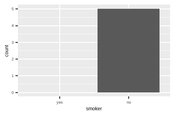
You can force them to display by supplying drop = FALSE to the appropriate discrete axis:
你可以通过向相应的离散坐标轴提供 drop = FALSE 来强制显示它们：

ggplot(health, aes(x = smoker)) +
  geom_bar() +
  scale_x_discrete()

ggplot(health, aes(x = smoker)) +
  geom_bar() +
  scale_x_discrete(drop = FALSE)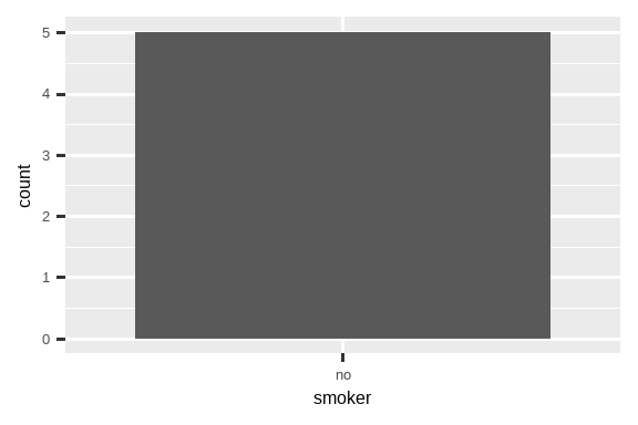

A bar chart with a single value on the x-axis, "no". The same bar chart as the last plot, but now with two values on the x-axis, "yes" and "no". There is no bar for the "yes" category.

The same problem comes up more generally with dplyr::group_by().
更普遍地，dplyr::group_by() 也会出现同样的问题。

And again you can use .drop = FALSE to preserve all factor levels:
同样，你可以使用 .drop = FALSE 来保留所有的因子水平：

health |> 
  group_by(smoker, .drop = FALSE) |> 
  summarize(
    n = n(),
    mean_age = mean(age),
    min_age = min(age),
    max_age = max(age),
    sd_age = sd(age)
  )
#> # A tibble: 2 × 6
#>   smoker     n mean_age min_age max_age sd_age
#>   <fct>  <int>    <dbl>   <dbl>   <dbl>  <dbl>
#> 1 yes        0      NaN     Inf    -Inf   NA  
#> 2 no         5       60      34      88   21.6

We get some interesting results here because when summarizing an empty group, the summary functions are applied to zero-length vectors.
我们在这里得到了一些有趣的结果，因为当对一个空组进行汇总时，汇总函数被应用于长度为零的向量。

There’s an important distinction between empty vectors, which have length 0, and missing values, each of which has length 1.
空向量（长度为 0）和缺失值（每个长度为 1）之间有一个重要的区别。

# A vector containing two missing values
x1 <- c(NA, NA)
length(x1)
#> [1] 2

# A vector containing nothing
x2 <- numeric()
length(x2)
#> [1] 0

All summary functions work with zero-length vectors, but they may return results that are surprising at first glance.
所有的汇总函数都可以处理零长度向量，但它们返回的结果乍一看可能会令人惊讶。

Here we see mean(age) returning NaN because mean(age) = sum(age)/length(age) which here is 0/0.
在这里我们看到 mean(age) 返回 NaN，因为 mean(age) = sum(age)/length(age)，在这里是 0/0。

max() and min() return -Inf and Inf for empty vectors so if you combine the results with a non-empty vector of new data and recompute you’ll get the minimum or maximum of the new data¹.
对于空向量，max() 和 min() 会返回 -Inf 和 Inf，所以如果你将结果与一个新的非空向量数据结合起来重新计算，你将得到新数据的最小值或最大值¹。

Sometimes a simpler approach is to perform the summary and then make the implicit missings explicit with complete().
有时，一个更简单的方法是先执行汇总，然后使用 complete() 将隐式缺失显式化。

health |> 
  group_by(smoker) |> 
  summarize(
    n = n(),
    mean_age = mean(age),
    min_age = min(age),
    max_age = max(age),
    sd_age = sd(age)
  ) |> 
  complete(smoker)
#> # A tibble: 2 × 6
#>   smoker     n mean_age min_age max_age sd_age
#>   <fct>  <int>    <dbl>   <dbl>   <dbl>  <dbl>
#> 1 yes       NA       NA      NA      NA   NA  
#> 2 no         5       60      34      88   21.6

The main drawback of this approach is that you get an NA for the count, even though you know that it should be zero.
这种方法的主要缺点是，尽管你知道计数应该为零，但你却得到了一个 NA。

18.5 Summary

Missing values are weird!
缺失值很奇怪！

Sometimes they’re recorded as an explicit NA but other times you only notice them by their absence.
有时它们被记录为显式的 NA，但其他时候你只能通过它们的缺席来注意到它们。

This chapter has given you some tools for working with explicit missing values, tools for uncovering implicit missing values, and discussed some of the ways that implicit can become explicit and vice versa.
本章为你提供了一些处理显式缺失值的工具，一些揭示隐式缺失值的工具，并讨论了隐式如何变为显式以及反之亦然的一些方法。

In the next chapter, we tackle the final chapter in this part of the book: joins.
在下一章中，我们将探讨本书这一部分的最后一章：连接 (joins)。

This is a bit of a change from the chapters so far because we’re going to discuss tools that work with data frames as a whole, not something that you put inside a data frame.
这与到目前为止的章节有些不同，因为我们将要讨论的是作用于整个数据框的工具，而不是你放在数据框内部的东西。

In other words, min(c(x, y)) is always equal to min(min(x), min(y)).↩︎