13 Numbers
13.1 Introduction
Numeric vectors are the backbone of data science, and you’ve already used them a bunch of times earlier in the book.
数值向量是数据科学的支柱,你已经在本书的前面部分多次使用过它们。
Now it’s time to systematically survey what you can do with them in R, ensuring that you’re well situated to tackle any future problem involving numeric vectors.
现在是时候系统地审视一下你可以用 R 对它们做什么,确保你能够很好地应对未来任何涉及数值向量的问题。
We’ll start by giving you a couple of tools to make numbers if you have strings, and then going into a little more detail of count().
我们将从介绍几个在你拥有字符串时用来创建数字的工具开始,然后更详细地探讨 count() 函数。
Then we’ll dive into various numeric transformations that pair well with mutate(), including more general transformations that can be applied to other types of vectors, but are often used with numeric vectors.
接着,我们将深入探讨与 mutate() 搭配使用的各种数值转换,包括那些可以应用于其他类型向量,但常用于数值向量的更通用的转换。
We’ll finish off by covering the summary functions that pair well with summarize() and show you how they can also be used with mutate().
最后,我们将介绍与 summarize() 搭配使用的摘要函数,并展示它们如何也能与 mutate() 一起使用。
13.1.1 Prerequisites
This chapter mostly uses functions from base R, which are available without loading any packages.
本章主要使用 base R 中的函数,这些函数无需加载任何包即可使用。
But we still need the tidyverse because we’ll use these base R functions inside of tidyverse functions like mutate() and filter().
但我们仍然需要 tidyverse,因为我们将在 tidyverse 函数如 mutate() 和 filter() 中使用这些 base R 函数。
Like in the last chapter, we’ll use real examples from nycflights13, as well as toy examples made with c() and tribble().
与上一章一样,我们将使用来自 nycflights13 的真实示例,以及用 c() 和 tribble() 创建的玩具示例。
13.2 Making numbers
In most cases, you’ll get numbers already recorded in one of R’s numeric types: integer or double.
在大多数情况下,你会得到已经以 R 的数值类型之一(整数或双精度浮点数)记录的数字。
In some cases, however, you’ll encounter them as strings, possibly because you’ve created them by pivoting from column headers or because something has gone wrong in your data import process.
然而,在某些情况下,你会遇到以字符串形式出现的数字,这可能是因为你是通过将列标题转置而创建的它们,或者是因为你的数据导入过程中出现了问题。
readr provides two useful functions for parsing strings into numbers: parse_double() and parse_number().
readr 提供了两个有用的函数用于将字符串解析为数字:parse_double() 和 parse_number()。
Use parse_double() when you have numbers that have been written as strings:
当你拥有以字符串形式书写的数字时,请使用 parse_double():
x <- c("1.2", "5.6", "1e3")
parse_double(x)
#> [1]    1.2    5.6 1000.0
Use parse_number() when the string contains non-numeric text that you want to ignore.
当字符串包含你想要忽略的非数字文本时,请使用 parse_number()。
This is particularly useful for currency data and percentages:
这对于处理货币数据和百分比特别有用:
x <- c("$1,234", "USD 3,513", "59%")
parse_number(x)
#> [1] 1234 3513   59
13.3 Counts
It’s surprising how much data science you can do with just counts and a little basic arithmetic, so dplyr strives to make counting as easy as possible with count().
令人惊讶的是,仅用计数和一点基本算术就能完成大量的数据科学工作,因此 dplyr 致力于通过 count() 函数使计数尽可能地简单。
This function is great for quick exploration and checks during analysis:
这个函数非常适合在分析过程中进行快速探索和检查:
flights |> count(dest)
#> # A tibble: 105 × 2
#>   dest      n
#>   <chr> <int>
#> 1 ABQ     254
#> 2 ACK     265
#> 3 ALB     439
#> 4 ANC       8
#> 5 ATL   17215
#> 6 AUS    2439
#> # ℹ 99 more rows
(Despite the advice in Chapter 4, we usually put count() on a single line because it’s usually used at the console for a quick check that a calculation is working as expected.)
(尽管在 Chapter 4 中有相关建议,我们通常将 count() 写在单行上,因为它通常在控制台中用于快速检查计算是否按预期工作。)
If you want to see the most common values, add sort = TRUE:
如果你想查看最常见的值,请添加 sort = TRUE:
flights |> count(dest, sort = TRUE)
#> # A tibble: 105 × 2
#>   dest      n
#>   <chr> <int>
#> 1 ORD   17283
#> 2 ATL   17215
#> 3 LAX   16174
#> 4 BOS   15508
#> 5 MCO   14082
#> 6 CLT   14064
#> # ℹ 99 more rows
And remember that if you want to see all the values, you can use |> View() or |> print(n = Inf).
并且记住,如果你想查看所有值,你可以使用 |> View() 或 |> print(n = Inf)。
You can perform the same computation “by hand” with group_by(), summarize() and n().
你可以使用 group_by()、summarize() 和 n() “手动” 执行相同的计算。
This is useful because it allows you to compute other summaries at the same time:
这很有用,因为它允许你同时计算其他摘要:
n() is a special summary function that doesn’t take any arguments and instead accesses information about the “current” group.n() 是一个特殊的摘要函数,它不接受任何参数,而是访问关于 “当前” 组的信息。
This means that it only works inside dplyr verbs:
这意味着它只能在 dplyr 动词内部工作:
n()
#> Error in `n()`:
#> ! Must only be used inside data-masking verbs like `mutate()`,
#>   `filter()`, and `group_by()`.
There are a couple of variants of n() and count() that you might find useful:n() 和 count() 有几个你可能会觉得有用的变体:
-
n_distinct(x)counts the number of distinct (unique) values of one or more variables.
For example, we could figure out which destinations are served by the most carriers:n_distinct(x)计算一个或多个变量的不重复(唯一)值的数量。 例如,我们可以找出哪些目的地有最多的航空公司使用:flights |> group_by(dest) |> summarize(carriers = n_distinct(carrier)) |> arrange(desc(carriers)) #> # A tibble: 105 × 2 #> dest carriers #> <chr> <int> #> 1 ATL 7 #> 2 BOS 7 #> 3 CLT 7 #> 4 ORD 7 #> 5 TPA 7 #> 6 AUS 6 #> # ℹ 99 more rows -
A weighted count is a sum. For example you could “count” the number of miles each plane flew:
加权计数是一个求和。 例如,你可以“计数”每架飞机飞行的英里数: -
Weighted counts are a common problem so
count()has awtargument that does the same thing:
加权计数是一个常见问题,因此count()有一个wt参数可以实现同样的功能:flights |> count(tailnum, wt = distance) -
You can count missing values by combining
sum()andis.na(). In theflightsdataset this represents flights that are cancelled:
你可以通过结合sum()和is.na()来统计缺失值的数量。 在flights数据集中,这表示被取消的航班:
13.3.1 Exercises
- How can you use
count()to count the number of rows with a missing value for a given variable? - Expand the following calls to
count()to instead usegroup_by(),summarize(), andarrange():flights |> count(dest, sort = TRUE)flights |> count(tailnum, wt = distance)
13.4 Numeric transformations
Transformation functions work well with mutate() because their output is the same length as the input.
转换函数与 mutate() 配合得很好,因为它们的输出长度与输入长度相同。
The vast majority of transformation functions are already built into base R.
绝大多数的转换函数都已内置在 base R 中。
It’s impractical to list them all so this section will show the most useful ones.
要列出所有这些函数是不切实际的,所以本节将展示最有用的那些。
As an example, while R provides all the trigonometric functions that you might dream of, we don’t list them here because they’re rarely needed for data science.
举个例子,虽然 R 提供了你可能梦想到的所有三角函数,但我们在这里不列出它们,因为它们在数据科学中很少需要。
13.4.1 Arithmetic and recycling rules
We introduced the basics of arithmetic (+, -, *, /, ^) in Chapter 2 and have used them a bunch since.
我们在 Chapter 2 中介绍了算术(+、-、*、/、^)的基础知识,并且从那以后已经大量使用它们。
These functions don’t need a huge amount of explanation because they do what you learned in grade school.
这些函数不需要大量的解释,因为它们做的就是你在小学学到的东西。
But we need to briefly talk about the recycling rules which determine what happens when the left and right hand sides have different lengths.
但是我们需要简要讨论一下循环规则 (recycling rules),它决定了当左右两侧长度不同时会发生什么。
This is important for operations like flights |> mutate(air_time = air_time / 60) because there are 336,776 numbers on the left of / but only one on the right.
这对于像 flights |> mutate(air_time = air_time / 60) 这样的操作很重要,因为 / 的左边有 336,776 个数字,而右边只有一个。
R handles mismatched lengths by recycling, or repeating, the short vector.
R 通过循环 (recycling) 或重复较短的向量来处理长度不匹配的情况。
We can see this in operation more easily if we create some vectors outside of a data frame:
如果我们创建一些数据框之外的向量,可以更容易地看到这个操作:
Generally, you only want to recycle single numbers (i.e. vectors of length 1), but R will recycle any shorter length vector.
通常,你只想循环利用单个数字(即长度为 1 的向量),但 R 会循环利用任何更短长度的向量。
It usually (but not always) gives you a warning if the longer vector isn’t a multiple of the shorter:
如果较长的向量不是较短向量的倍数,它通常(但并非总是)会给你一个警告:
These recycling rules are also applied to logical comparisons (==, <, <=, >, >=, !=) and can lead to a surprising result if you accidentally use == instead of %in% and the data frame has an unfortunate number of rows.
这些循环规则也适用于逻辑比较(==、<、<=、>、>=、!=),如果你不小心使用了 == 而不是 %in%,并且数据框的行数不凑巧,可能会导致令人惊讶的结果。
For example, take this code which attempts to find all flights in January and February:
例如,看这段试图查找一月和二月所有航班的代码:
flights |>
  filter(month == c(1, 2))
#> # A tibble: 25,977 × 19
#>    year month   day dep_time sched_dep_time dep_delay arr_time sched_arr_time
#>   <int> <int> <int>    <int>          <int>     <dbl>    <int>          <int>
#> 1  2013     1     1      517            515         2      830            819
#> 2  2013     1     1      542            540         2      923            850
#> 3  2013     1     1      554            600        -6      812            837
#> 4  2013     1     1      555            600        -5      913            854
#> 5  2013     1     1      557            600        -3      838            846
#> 6  2013     1     1      558            600        -2      849            851
#> # ℹ 25,971 more rows
#> # ℹ 11 more variables: arr_delay <dbl>, carrier <chr>, flight <int>, …
The code runs without error, but it doesn’t return what you want.
代码运行没有错误,但它没有返回你想要的结果。
Because of the recycling rules it finds flights in odd numbered rows that departed in January and flights in even numbered rows that departed in February.
由于循环规则,它会查找奇数行中在一月出发的航班和偶数行中在二月出发的航班。
And unfortunately there’s no warning because flights has an even number of rows.
而且不幸的是,因为 flights 数据框有偶数行,所以没有警告。
To protect you from this type of silent failure, most tidyverse functions use a stricter form of recycling that only recycles single values.
为了保护你免受这类静默失败的影响,大多数 tidyverse 函数使用一种更严格的循环形式,只循环单个值。
Unfortunately that doesn’t help here, or in many other cases, because the key computation is performed by the base R function ==, not filter().
不幸的是,这在这里或许多其他情况下没有帮助,因为关键的计算是由 base R 函数 == 执行的,而不是 filter()。
13.4.2 Minimum and maximum
The arithmetic functions work with pairs of variables.
算术函数处理成对的变量。
Two closely related functions are pmin() and pmax(), which when given two or more variables will return the smallest or largest value in each row:
两个密切相关的函数是 pmin() 和 pmax(),当给定两个或多个变量时,它们将返回每行中的最小值或最大值:
Note that these are different to the summary functions min() and max() which take multiple observations and return a single value.
请注意,这些函数与摘要函数 min() 和 max() 不同,后者接受多个观测值并返回单个值。
You can tell that you’ve used the wrong form when all the minimums and all the maximums have the same value:
当所有的最小值和所有的最大值都具有相同的值时,你就可以判断出你使用了错误的形式:
13.4.3 Modular arithmetic
Modular arithmetic is the technical name for the type of math you did before you learned about decimal places, i.e. division that yields a whole number and a remainder.
模运算是你在学习小数之前所做的那种数学的专业术语,即产生整数和余数的除法。
In R, %/% does integer division and %% computes the remainder:
在 R 中,%/% 执行整数除法,而 %% 计算余数:
Modular arithmetic is handy for the flights dataset, because we can use it to unpack the sched_dep_time variable into hour and minute:
模运算对于 flights 数据集非常方便,因为我们可以用它将 sched_dep_time 变量分解为 hour 和 minute:
We can combine that with the mean(is.na(x)) trick from Section 12.4 to see how the proportion of cancelled flights varies over the course of the day.
我们可以将其与 Section 12.4 中的 mean(is.na(x)) 技巧结合起来,看看取消航班的比例在一天中是如何变化的。
The results are shown in Figure 13.1.
结果显示在 Figure 13.1 中。
flights |>
  group_by(hour = sched_dep_time %/% 100) |>
  summarize(prop_cancelled = mean(is.na(dep_time)), n = n()) |>
  filter(hour > 1) |>
  ggplot(aes(x = hour, y = prop_cancelled)) +
  geom_line(color = "grey50") +
  geom_point(aes(size = n))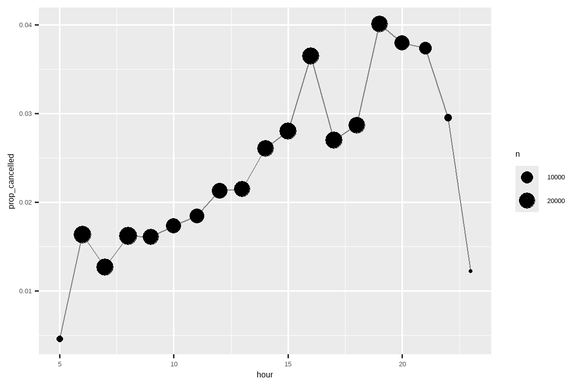
13.4.4 Logarithms
Logarithms are an incredibly useful transformation for dealing with data that ranges across multiple orders of magnitude and converting exponential growth to linear growth.
对数是一种非常有用的转换,用于处理跨越多个数量级的数据,并将指数增长转换为线性增长。
In R, you have a choice of three logarithms: log() (the natural log, base e), log2() (base 2), and log10() (base 10).
在 R 中,你可以选择三种对数:log() (自然对数,以 e 为底)、log2() (以 2 为底) 和 log10() (以 10 为底)。
We recommend using log2() or log10().
我们推荐使用 log2() 或 log10()。
log2() is easy to interpret because a difference of 1 on the log scale corresponds to doubling on the original scale and a difference of -1 corresponds to halving; whereas log10() is easy to back-transform because (e.g.) 3 is 10^3 = 1000.log2() 很容易解释,因为对数尺度上的 1 个单位差异对应于原始尺度上的加倍,而 -1 的差异则对应于减半;而 log10() 很容易进行逆转换,因为(例如)3 是 10^3 = 1000。
The inverse of log() is exp(); to compute the inverse of log2() or log10() you’ll need to use 2^ or 10^.log() 的逆运算是 exp();要计算 log2() 或 log10() 的逆运算,你需要使用 2^ 或 10^。
13.4.5 Rounding
Use round(x) to round a number to the nearest integer:
使用 round(x) 将数字四舍五入到最接近的整数:
round(123.456)
#> [1] 123
You can control the precision of the rounding with the second argument, digits.
你可以使用第二个参数 digits 来控制四舍五入的精度。
round(x, digits) rounds to the nearest 10^-n so digits = 2 will round to the nearest 0.01.round(x, digits) 会四舍五入到最接近的 10^-n,所以 digits = 2 会四舍五入到最接近的 0.01。
This definition is useful because it implies round(x, -3) will round to the nearest thousand, which indeed it does:
这个定义很有用,因为它意味着 round(x, -3) 会四舍五入到最接近的千位,事实也确实如此:
There’s one weirdness with round() that seems surprising at first glance:round() 有一个乍一看似乎很奇怪的特性:
round() uses what’s known as “round half to even” or Banker’s rounding: if a number is half way between two integers, it will be rounded to the even integer.round() 使用所谓的 “四舍六入五成双” 或银行家舍入法:如果一个数字正好在两个整数中间,它将被舍入到偶数。
This is a good strategy because it keeps the rounding unbiased: half of all 0.5s are rounded up, and half are rounded down.
这是一个很好的策略,因为它能保持舍入的无偏性:一半的 0.5 会向上舍入,一半会向下舍入。
round() is paired with floor() which always rounds down and ceiling() which always rounds up:round() 与 floor()(总是向下取整)和 ceiling()(总是向上取整)配对使用:
These functions don’t have a digits argument, so you can instead scale down, round, and then scale back up:
这些函数没有 digits 参数,所以你可以先缩小,然后取整,再放大回去:
You can use the same technique if you want to round() to a multiple of some other number:
如果你想 round() 到某个其他数字的倍数,也可以使用相同的技巧:
13.4.6 Cutting numbers into ranges
Use cut()1 to break up (aka bin) a numeric vector into discrete buckets:
使用 cut()1 将一个数值向量分割(也称分箱)成离散的区间:
The breaks don’t need to be evenly spaced:
分割点不需要均匀分布:
You can optionally supply your own labels.
你可以选择性地提供自己的 labels。
Note that there should be one less labels than breaks.
请注意,labels 的数量应该比 breaks 少一个。
Any values outside of the range of the breaks will become NA:
任何超出分割点范围的值都将变为 NA:
See the documentation for other useful arguments like right and include.lowest, which control if the intervals are [a, b) or (a, b] and if the lowest interval should be [a, b].
请参阅文档以了解其他有用的参数,如 right 和 include.lowest,它们控制区间是 [a, b) 还是 (a, b],以及最低的区间是否应为 [a, b]。
13.4.7 Cumulative and rolling aggregates
Base R provides cumsum(), cumprod(), cummin(), cummax() for running, or cumulative, sums, products, mins and maxes.
Base R 提供了 cumsum()、cumprod()、cummin()、cummax() 用于计算游动或累积的和、积、最小值和最大值。
dplyr provides cummean() for cumulative means.
dplyr 提供了 cummean() 用于计算累积均值。
Cumulative sums tend to come up the most in practice:
累积和在实践中最为常见:
x <- 1:10
cumsum(x)
#>  [1]  1  3  6 10 15 21 28 36 45 55
If you need more complex rolling or sliding aggregates, try the slider package.
如果你需要更复杂的滚动或滑动聚合,可以试试 slider 包。
13.4.8 Exercises
Explain in words what each line of the code used to generate Figure 13.1 does.
What trigonometric functions does R provide? Guess some names and look up the documentation. Do they use degrees or radians?
-
Currently
dep_timeandsched_dep_timeare convenient to look at, but hard to compute with because they’re not really continuous numbers. You can see the basic problem by running the code below: there’s a gap between each hour.flights |> filter(month == 1, day == 1) |> ggplot(aes(x = sched_dep_time, y = dep_delay)) + geom_point()Convert them to a more truthful representation of time (either fractional hours or minutes since midnight).
Round
dep_timeandarr_timeto the nearest five minutes.
13.5 General transformations
The following sections describe some general transformations which are often used with numeric vectors, but can be applied to all other column types.
以下各节描述了一些通常用于数值向量,但也可以应用于所有其他列类型的一般转换。
13.5.1 Ranks
dplyr provides a number of ranking functions inspired by SQL, but you should always start with dplyr::min_rank().
dplyr 提供了一些受 SQL 启发的排名函数,但你应该总是从 dplyr::min_rank() 开始。
It uses the typical method for dealing with ties, e.g., 1st, 2nd, 2nd, 4th.
它使用处理平局的典型方法,例如,第 1 名、第 2 名、第 2 名、第 4 名。
Note that the smallest values get the lowest ranks; use desc(x) to give the largest values the smallest ranks:
注意,最小值获得最低的排名;使用 desc(x) 可以让最大值获得最低的排名:
If min_rank() doesn’t do what you need, look at the variants dplyr::row_number(), dplyr::dense_rank(), dplyr::percent_rank(), and dplyr::cume_dist().
如果 min_rank() 不能满足你的需求,可以看看它的变体 dplyr::row_number()、dplyr::dense_rank()、dplyr::percent_rank() 和 dplyr::cume_dist()。
See the documentation for details.
详情请参阅文档。
df <- tibble(x = x)
df |>
  mutate(
    row_number = row_number(x),
    dense_rank = dense_rank(x),
    percent_rank = percent_rank(x),
    cume_dist = cume_dist(x)
  )
#> # A tibble: 6 × 5
#>       x row_number dense_rank percent_rank cume_dist
#>   <dbl>      <int>      <int>        <dbl>     <dbl>
#> 1     1          1          1         0          0.2
#> 2     2          2          2         0.25       0.6
#> 3     2          3          2         0.25       0.6
#> 4     3          4          3         0.75       0.8
#> 5     4          5          4         1          1
#> 6    NA         NA         NA        NA         NA
You can achieve many of the same results by picking the appropriate ties.method argument to base R’s rank(); you’ll probably also want to set na.last = "keep" to keep NAs as NA.
通过为 base R 的 rank() 函数选择合适的 ties.method 参数,你可以实现许多相同的结果;你可能还想设置 na.last = "keep" 以将 NA 保留为 NA。
row_number() can also be used without any arguments when inside a dplyr verb.row_number() 在 dplyr 动词内部使用时也可以不带任何参数。
In this case, it’ll give the number of the “current” row.
在这种情况下,它会给出 “当前” 行的行号。
When combined with %% or %/% this can be a useful tool for dividing data into similarly sized groups:
当与 %% 或 %/% 结合使用时,这可以成为将数据划分为大小相近的组的有用工具:
df <- tibble(id = 1:10)

df |>
  mutate(
    row0 = row_number() - 1,
    three_groups = row0 %% 3,
    three_in_each_group = row0 %/% 3
  )
#> # A tibble: 10 × 4
#>      id  row0 three_groups three_in_each_group
#>   <int> <dbl>        <dbl>               <dbl>
#> 1     1     0            0                   0
#> 2     2     1            1                   0
#> 3     3     2            2                   0
#> 4     4     3            0                   1
#> 5     5     4            1                   1
#> 6     6     5            2                   1
#> # ℹ 4 more rows
13.5.2 Offsets
dplyr::lead() and dplyr::lag() allow you to refer to the values just before or just after the “current” value.dplyr::lead() 和 dplyr::lag() 允许你引用 “当前” 值之前或之后的值。
They return a vector of the same length as the input, padded with NAs at the start or end:
它们返回一个与输入长度相同的向量,在开头或结尾用 NA 填充:
-
x - lag(x)gives you the difference between the current and previous value.x - lag(x)给出当前值与前一个值之间的差异。x - lag(x) #> [1] NA 3 6 0 8 16`
-
x == lag(x)tells you when the current value changes.x == lag(x)告诉你当前值何时发生变化。x == lag(x) #> [1] NA FALSE FALSE TRUE FALSE FALSE
You can lead or lag by more than one position by using the second argument, n.
你可以通过使用第二个参数 n 来前导或滞后超过一个位置。
13.5.3 Consecutive identifiers
Sometimes you want to start a new group every time some event occurs.
有时你希望在每次某个事件发生时开始一个新的组。
For example, when you’re looking at website data, it’s common to want to break up events into sessions, where you begin a new session after a gap of more than x minutes since the last activity.
例如,在查看网站数据时,通常希望将事件分解为会话 (sessions),即在距离上次活动超过 x 分钟后开始一个新的会话。
For example, imagine you have the times when someone visited a website:
例如,假设你有一个人访问网站的时间记录:
And you’ve computed the time between each event, and figured out if there’s a gap that’s big enough to qualify:
并且你已经计算了每个事件之间的时间,并判断是否存在足够大的间隔:
But how do we go from that logical vector to something that we can group_by()?
但是我们如何从那个逻辑向量转变为可以用于 group_by() 的东西呢?
cumsum(), from Section 13.4.7, comes to the rescue as gap, i.e. has_gap is TRUE, will increment group by one (Section 12.4.2):
来自 Section 13.4.7 的 cumsum() 此时就派上用场了,因为当间隙存在时,即 has_gap 为 TRUE,group 将会加一 (Section 12.4.2):
Another approach for creating grouping variables is consecutive_id(), which starts a new group every time one of its arguments changes.
另一种创建分组变量的方法是 consecutive_id(),它在每次其参数之一发生变化时开始一个新的组。
For example, inspired by this stackoverflow question, imagine you have a data frame with a bunch of repeated values:
例如,受 这个 stackoverflow 问题 的启发,想象你有一个包含许多重复值的数据框:
If you want to keep the first row from each repeated x, you could use group_by(), consecutive_id(), and slice_head():
如果你想保留每个重复 x 的第一行,你可以使用 group_by()、consecutive_id() 和 slice_head():
df |>
  group_by(id = consecutive_id(x)) |>
  slice_head(n = 1)
#> # A tibble: 7 × 3
#> # Groups:   id [7]
#>   x         y    id
#>   <chr> <dbl> <int>
#> 1 a         1     1
#> 2 b         2     2
#> 3 c         4     3
#> 4 d         3     4
#> 5 e         9     5
#> 6 a         4     6
#> # ℹ 1 more row
13.5.4 Exercises
Find the 10 most delayed flights using a ranking function. How do you want to handle ties? Carefully read the documentation for
min_rank().Which plane (
tailnum) has the worst on-time record?What time of day should you fly if you want to avoid delays as much as possible?
What does
flights |> group_by(dest) |> filter(row_number() < 4)do? What doesflights |> group_by(dest) |> filter(row_number(dep_delay) < 4)do?For each destination, compute the total minutes of delay. For each flight, compute the proportion of the total delay for its destination.
-
Delays are typically temporally correlated: even once the problem that caused the initial delay has been resolved, later flights are delayed to allow earlier flights to leave. Using
lag(), explore how the average flight delay for an hour is related to the average delay for the previous hour. Look at each destination. Can you find flights that are suspiciously fast (i.e. flights that represent a potential data entry error)? Compute the air time of a flight relative to the shortest flight to that destination. Which flights were most delayed in the air?
Find all destinations that are flown by at least two carriers. Use those destinations to come up with a relative ranking of the carriers based on their performance for the same destination.
13.6 Numeric summaries
Just using the counts, means, and sums that we’ve introduced already can get you a long way, but R provides many other useful summary functions.
仅使用我们已经介绍过的计数、均值和总和就可以让你走得很远,但 R 提供了许多其他有用的摘要函数。
Here is a selection that you might find useful.
这里是一些你可能会觉得有用的选择。
13.6.1 Center
So far, we’ve mostly used mean() to summarize the center of a vector of values.
到目前为止,我们主要使用 mean() 来概括一个数值向量的中心。
As we’ve seen in Section 3.6, because the mean is the sum divided by the count, it is sensitive to even just a few unusually high or low values.
正如我们在 Section 3.6 中看到的,因为均值是总和除以计数,所以它对哪怕是少数几个异常高或低的值都很敏感。
An alternative is to use the median(), which finds a value that lies in the “middle” of the vector, i.e. 50% of the values are above it and 50% are below it.
另一种方法是使用 median(),它会找到一个位于向量“中间”的值,即 50% 的值在它之上,50% 的值在它之下。
Depending on the shape of the distribution of the variable you’re interested in, mean or median might be a better measure of center.
根据你所关心变量的分布形状,均值或中位数可能是更好的中心度量。
For example, for symmetric distributions we generally report the mean while for skewed distributions we usually report the median.
例如,对于对称分布,我们通常报告均值,而对于偏态分布,我们通常报告中位数。
Figure 13.2 compares the mean vs. the median departure delay (in minutes) for each destination.
Figure 13.2 比较了每个目的地的平均出发延迟(分钟)与中位数出发延迟。
The median delay is always smaller than the mean delay because flights sometimes leave multiple hours late, but never leave multiple hours early.
中位数延迟总是小于平均延迟,因为航班有时会晚点数小时,但从不会提前数小时出发。
flights |>
  group_by(year, month, day) |>
  summarize(
    mean = mean(dep_delay, na.rm = TRUE),
    median = median(dep_delay, na.rm = TRUE),
    n = n(),
    .groups = "drop"
  ) |>
  ggplot(aes(x = mean, y = median)) +
  geom_abline(slope = 1, intercept = 0, color = "white", linewidth = 2) +
geom_point()![All points fall below a 45° line, meaning that the median delay is always less than the mean delay. Most points are clustered in a dense region of mean [0, 20] and median [-5, 5]. As the mean delay increases, the spread of the median also increases. There are two outlying points with mean ~60, median ~30, and mean ~85, median ~55.](numbers_files/figure-html/fig-mean-vs-median-1.png)
You might also wonder about the mode, or the most common value.
你可能还会想知道众数,即最常见的值。
This is a summary that only works well for very simple cases (which is why you might have learned about it in high school), but it doesn’t work well for many real datasets.
这是一个只在非常简单的情况下才有效的摘要(这就是为什么你可能在高中学过它),但它对许多真实数据集效果不佳。
If the data is discrete, there may be multiple most common values, and if the data is continuous, there might be no most common value because every value is ever so slightly different.
如果数据是离散的,可能会有多个最常见的值;如果数据是连续的,可能没有最常见的值,因为每个值都略有不同。
For these reasons, the mode tends not to be used by statisticians and there’s no mode function included in base R2.
由于这些原因,统计学家倾向于不使用众数,并且 base R 中没有包含众数函数2。
13.6.2 Minimum, maximum, and quantiles
What if you’re interested in locations other than the center?
如果你对中心以外的位置感兴趣怎么办?
min() and max() will give you the largest and smallest values.min() 和 max() 会给你最大值和最小值。
Another powerful tool is quantile() which is a generalization of the median: quantile(x, 0.25) will find the value of x that is greater than 25% of the values, quantile(x, 0.5) is equivalent to the median, and quantile(x, 0.95) will find the value that’s greater than 95% of the values.
另一个强大的工具是 quantile(),它是中位数的推广:quantile(x, 0.25) 将找到 x 中大于 25% 值的值,quantile(x, 0.5) 等同于中位数,而 quantile(x, 0.95) 将找到大于 95% 值的值。
For the flights data, you might want to look at the 95% quantile of delays rather than the maximum, because it will ignore the 5% of most delayed flights which can be quite extreme.
对于 flights 数据,你可能想查看延迟的 95% 分位数而不是最大值,因为它会忽略最延迟的 5% 航班,这些航班可能非常极端。
flights |>
  group_by(year, month, day) |>
  summarize(
    max = max(dep_delay, na.rm = TRUE),
    q95 = quantile(dep_delay, 0.95, na.rm = TRUE),
    .groups = "drop"
  )
#> # A tibble: 365 × 5
#>    year month   day   max   q95
#>   <int> <int> <int> <dbl> <dbl>
#> 1  2013     1     1   853  70.1
#> 2  2013     1     2   379  85
#> 3  2013     1     3   291  68
#> 4  2013     1     4   288  60
#> 5  2013     1     5   327  41
#> 6  2013     1     6   202  51
#> # ℹ 359 more rows
13.6.3 Spread
Sometimes you’re not so interested in where the bulk of the data lies, but in how it is spread out.
有时你不太关心数据的主体在哪里,而关心它是如何分布的。
Two commonly used summaries are the standard deviation, sd(x), and the inter-quartile range, IQR().
两个常用的摘要是标准差 sd(x) 和四分位距 IQR()。
We won’t explain sd() here since you’re probably already familiar with it, but IQR() might be new — it’s quantile(x, 0.75) - quantile(x, 0.25) and gives you the range that contains the middle 50% of the data.
我们在这里不会解释 sd(),因为你可能已经熟悉它了,但 IQR() 可能对你来说是新的——它是 quantile(x, 0.75) - quantile(x, 0.25),并给出包含中间 50% 数据的范围。
We can use this to reveal a small oddity in the flights data.
我们可以用这个来揭示 flights 数据中的一个小小的奇特之处。
You might expect the spread of the distance between origin and destination to be zero, since airports are always in the same place.
你可能期望始发地和目的地之间距离的离散程度为零,因为机场总是在同一个地方。
But the code below reveals a data oddity for airport EGE:
但是下面的代码揭示了关于 EGE 机场的一个数据异常:
13.6.4 Distributions
It’s worth remembering that all of the summary statistics described above are a way of reducing the distribution down to a single number.
值得记住的是,上面描述的所有摘要统计量都是将分布简化为单个数字的一种方式。
This means that they’re fundamentally reductive, and if you pick the wrong summary, you can easily miss important differences between groups.
这意味着它们在根本上是简化的,如果你选择了错误的摘要,你很容易会错过组间的重要差异。
That’s why it’s always a good idea to visualize the distribution before committing to your summary statistics.
这就是为什么在确定你的摘要统计数据之前,可视化分布总是一个好主意。
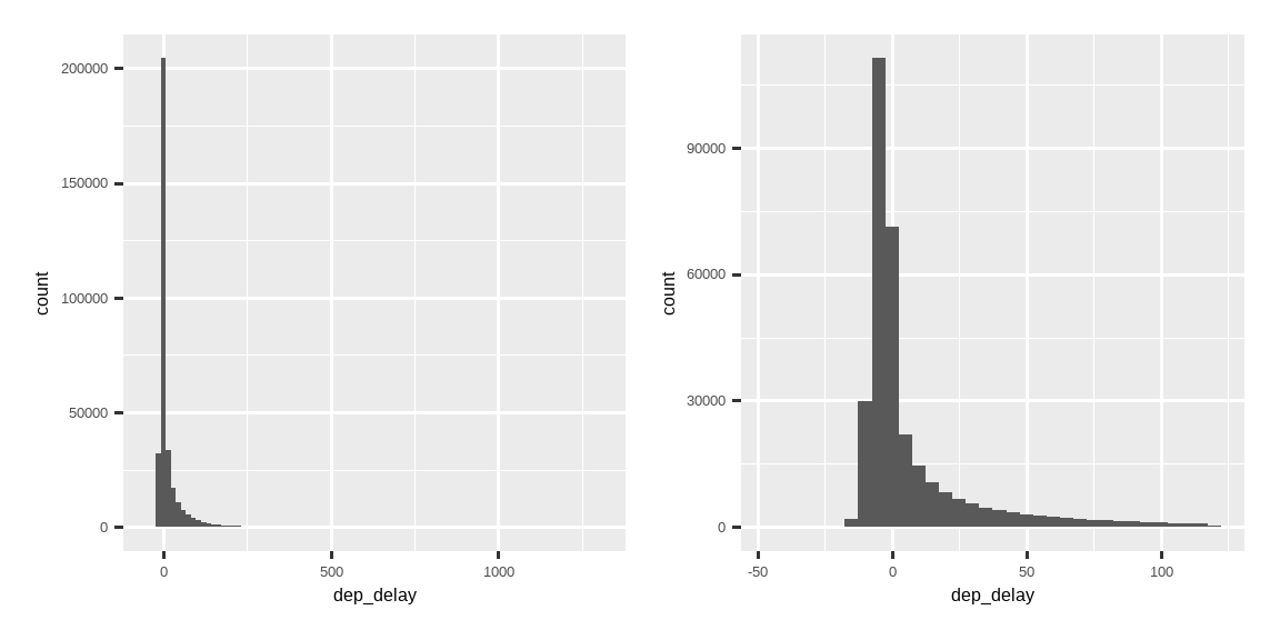
Figure 13.3 shows the overall distribution of departure delays.
Figure 13.3 显示了出发延误的总体分布。
The distribution is so skewed that we have to zoom in to see the bulk of the data.
该分布非常偏斜,以至于我们必须放大才能看到数据的主体部分。
This suggests that the mean is unlikely to be a good summary and we might prefer the median instead.
这表明均值不太可能是一个好的摘要,我们可能更倾向于使用中位数。
It’s also a good idea to check that distributions for subgroups resemble the whole.
检查子组的分布是否与整体相似也是一个好主意。
In the following plot 365 frequency polygons of dep_delay, one for each day, are overlaid.
在下面的图中,叠加了 365 个 dep_delay 的频率多边形,每天一个。
The distributions seem to follow a common pattern, suggesting it’s fine to use the same summary for each day.
这些分布似乎遵循一个共同的模式,这表明每天使用相同的摘要是可以的。
flights |>
  filter(dep_delay < 120) |>
  ggplot(aes(x = dep_delay, group = interaction(day, month))) +
  geom_freqpoly(binwidth = 5, alpha = 1/5)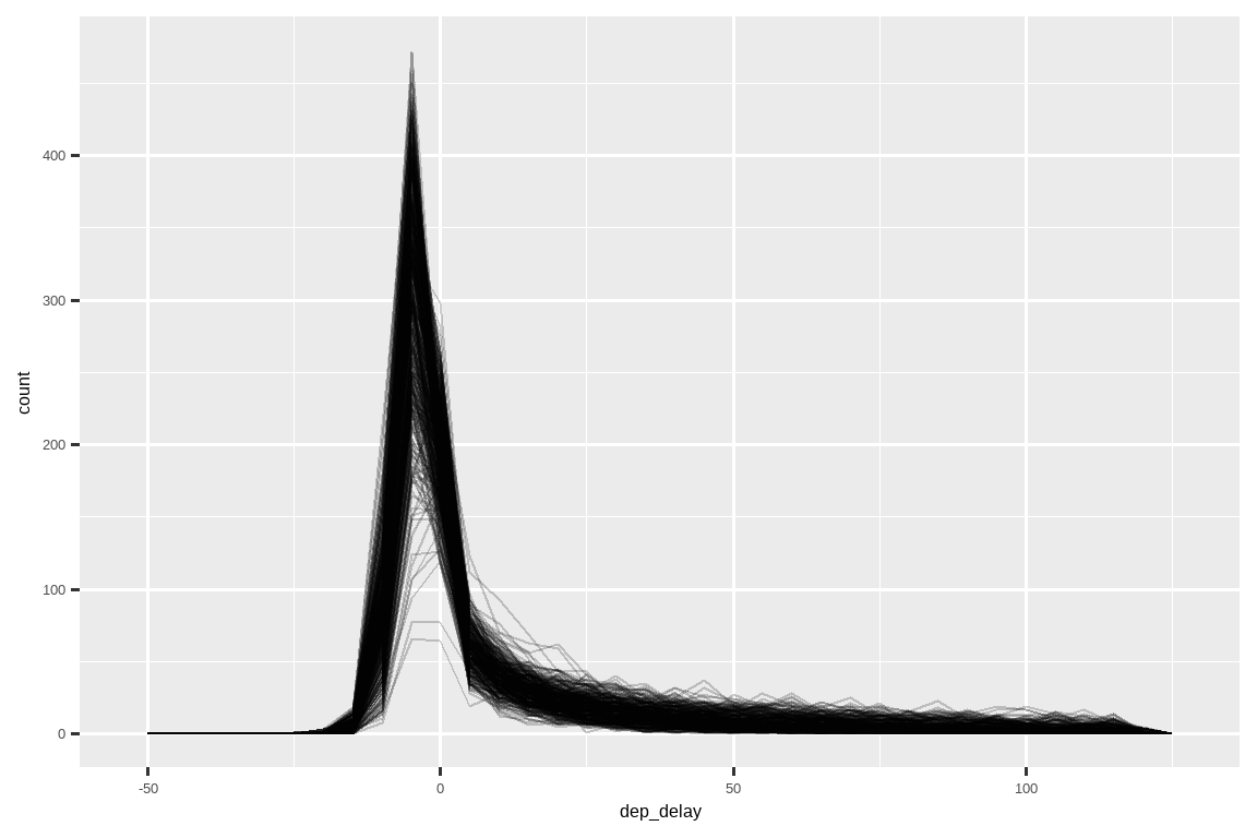
Don’t be afraid to explore your own custom summaries specifically tailored for the data that you’re working with.
不要害怕探索为你正在处理的数据量身定制的自定义摘要。
In this case, that might mean separately summarizing the flights that left early vs. the flights that left late, or given that the values are so heavily skewed, you might try a log-transformation.
在这种情况下,这可能意味着分别总结提前起飞的航班和晚点起飞的航班,或者鉴于数值偏斜严重,你可以尝试进行对数转换。
Finally, don’t forget what you learned in Section 3.6: whenever creating numerical summaries, it’s a good idea to include the number of observations in each group.
最后,别忘了你在 Section 3.6 中学到的:每当创建数值摘要时,最好包含每个组中的观测数量。
13.6.5 Positions
There’s one final type of summary that’s useful for numeric vectors, but also works with every other type of value: extracting a value at a specific position: first(x), last(x), and nth(x, n).
还有最后一种对数值向量很有用,但也适用于所有其他类型值的摘要:提取特定位置的值:first(x)、last(x) 和 nth(x, n)。
For example, we can find the first, fifth and last departure for each day:
例如,我们可以找到每天的第一次、第五次和最后一次出发:
flights |>
  group_by(year, month, day) |>
  summarize(
    first_dep = first(dep_time, na_rm = TRUE),
    fifth_dep = nth(dep_time, 5, na_rm = TRUE),
    last_dep = last(dep_time, na_rm = TRUE)
  )
#> `summarise()` has grouped output by 'year', 'month'. You can override using
#> the `.groups` argument.
#> # A tibble: 365 × 6
#> # Groups:   year, month [12]
#>    year month   day first_dep fifth_dep last_dep
#>   <int> <int> <int>     <int>     <int>    <int>
#> 1  2013     1     1       517       554     2356
#> 2  2013     1     2        42       535     2354
#> 3  2013     1     3        32       520     2349
#> 4  2013     1     4        25       531     2358
#> 5  2013     1     5        14       534     2357
#> 6  2013     1     6        16       555     2355
#> # ℹ 359 more rows
(NB: Because dplyr functions use _ to separate components of function and arguments names, these functions use na_rm instead of na.rm.)
(注意:因为 dplyr 函数使用 _ 来分隔函数和参数名称的组成部分,所以这些函数使用 na_rm 而不是 na.rm。)
If you’re familiar with [, which we’ll come back to in Section 27.2, you might wonder if you ever need these functions.
如果你熟悉 [(我们将在 Section 27.2 中回过头来讨论),你可能会想知道你是否真的需要这些函数。
There are three reasons: the default argument allows you to provide a default if the specified position doesn’t exist, the order_by argument allows you to locally override the order of the rows, and the na_rm argument allows you to drop missing values.
有三个原因:default 参数允许你在指定位置不存在时提供一个默认值,order_by 参数允许你局部覆盖行的顺序,而 na_rm 参数允许你删除缺失值。
Extracting values at positions is complementary to filtering on ranks.
按位置提取值与按排名筛选是互补的。
Filtering gives you all variables, with each observation in a separate row:
筛选会给你所有变量,每个观测值占一行:
flights |>
  group_by(year, month, day) |>
  mutate(r = min_rank(sched_dep_time)) |>
  filter(r %in% c(1, max(r)))
#> # A tibble: 1,195 × 20
#> # Groups:   year, month, day [365]
#>    year month   day dep_time sched_dep_time dep_delay arr_time sched_arr_time
#>   <int> <int> <int>    <int>          <int>     <dbl>    <int>          <int>
#> 1  2013     1     1      517            515         2      830            819
#> 2  2013     1     1     2353           2359        -6      425            445
#> 3  2013     1     1     2353           2359        -6      418            442
#> 4  2013     1     1     2356           2359        -3      425            437
#> 5  2013     1     2       42           2359        43      518            442
#> 6  2013     1     2      458            500        -2      703            650
#> # ℹ 1,189 more rows
#> # ℹ 12 more variables: arr_delay <dbl>, carrier <chr>, flight <int>, …
13.6.6 With mutate()
As the names suggest, the summary functions are typically paired with summarize().
正如其名,摘要函数通常与 summarize() 配对使用。
However, because of the recycling rules we discussed in Section 13.4.1 they can also be usefully paired with mutate(), particularly when you want do some sort of group standardization.
然而,由于我们在 Section 13.4.1 中讨论的循环规则,它们也可以与 mutate() 有效地配对,特别是当你想要进行某种分组标准化时。
For example:
例如:
x / sum(x)calculates the proportion of a total.x / sum(x)计算占总数的比例。(x - mean(x)) / sd(x)computes a Z-score (standardized to mean 0 and sd 1).(x - mean(x)) / sd(x)计算一个 Z 分数(标准化为均值为 0,标准差为 1)。(x - min(x)) / (max(x) - min(x))standardizes to range [0, 1].(x - min(x)) / (max(x) - min(x))将数据标准化到 [0, 1] 范围。x / first(x)computes an index based on the first observation.x / first(x)根据第一个观测值计算一个指数。
13.6.7 Exercises
Brainstorm at least 5 different ways to assess the typical delay characteristics of a group of flights. When is
mean()useful? When ismedian()useful? When might you want to use something else? Should you use arrival delay or departure delay? Why might you want to use data fromplanes?Which destinations show the greatest variation in air speed?
Create a plot to further explore the adventures of EGE. Can you find any evidence that the airport moved locations? Can you find another variable that might explain the difference?
13.7 Summary
You’re already familiar with many tools for working with numbers, and after reading this chapter you now know how to use them in R.
你已经熟悉许多处理数字的工具,在阅读本章后,你现在知道如何在 R 中使用它们了。
You’ve also learned a handful of useful general transformations that are commonly, but not exclusively, applied to numeric vectors like ranks and offsets.
你还学到了一些有用的通用转换,它们通常(但非唯一)应用于像排名和偏移量这样的数值向量。
Finally, you worked through a number of numeric summaries, and discussed a few of the statistical challenges that you should consider.
最后,你学习了一些数值摘要,并讨论了一些你应该考虑的统计挑战。
Over the next two chapters, we’ll dive into working with strings with the stringr package.
在接下来的两章中,我们将深入探讨使用 stringr 包处理字符串。
Strings are a big topic so they get two chapters, one on the fundamentals of strings and one on regular expressions.
字符串是一个很大的主题,所以它们有两章的篇幅,一章关于字符串的基础知识,另一章关于正则表达式。
ggplot2 provides some helpers for common cases in
cut_interval(),cut_number(), andcut_width(). ggplot2 is an admittedly weird place for these functions to live, but they are useful as part of histogram computation and were written before any other parts of the tidyverse existed.↩︎