27 A field guide to base R
27.1 Introduction
To finish off the programming section, we’re going to give you a quick tour of the most important base R functions that we don’t otherwise discuss in the book.
为了结束编程部分,我们将带你快速浏览一下本书中未曾讨论过的最重要的基础 R 函数。
These tools are particularly useful as you do more programming and will help you read code you’ll encounter in the wild.
当你进行更多编程时,这些工具特别有用,它们将帮助你阅读在实际中遇到的代码。
This is a good place to remind you that the tidyverse is not the only way to solve data science problems.
这里正好可以提醒你,tidyverse 并不是解决数据科学问题的唯一方法。
We teach the tidyverse in this book because tidyverse packages share a common design philosophy, increasing the consistency across functions, and making each new function or package a little easier to learn and use.
我们在本书中教授 tidyverse,因为 tidyverse 的包共享一个共同的设计理念,增加了函数之间的一致性,使得学习和使用每个新函数或包都变得更容易一些。
It’s not possible to use the tidyverse without using base R, so we’ve actually already taught you a lot of base R functions: from library() to load packages, to sum() and mean() for numeric summaries, to the factor, date, and POSIXct data types, and of course all the basic operators like +, -, /, *, |, &, and !.
不使用基础 R 是不可能使用 tidyverse 的,所以我们实际上已经教了你很多基础 R 函数:从加载包的 library(),到用于数值摘要的 sum() 和 mean(),再到因子、日期和 POSIXct 数据类型,当然还有所有基本运算符,如 +、-、/、*、|、& 和 !。
What we haven’t focused on so far is base R workflows, so we will highlight a few of those in this chapter.
到目前为止,我们还没有重点关注基础 R 的工作流程,所以我们将在本章中重点介绍其中的一些。
After you read this book, you’ll learn other approaches to the same problems using base R, data.table, and other packages.
读完这本书后,你将学习到使用基础 R、data.table 和其他包来解决同样问题的其他方法。
You’ll undoubtedly encounter these other approaches when you start reading R code written by others, particularly if you’re using StackOverflow.
当你开始阅读他人编写的 R 代码时,毫无疑问你会遇到这些其他方法,尤其是在使用 StackOverflow 时。
It’s 100% okay to write code that uses a mix of approaches, and don’t let anyone tell you otherwise!
编写混合使用多种方法的代码是 100% 可以的,不要让任何人告诉你别的!
In this chapter, we’ll focus on four big topics: subsetting with [, subsetting with [[ and $, the apply family of functions, and for loops.
在本章中,我们将重点关注四个大主题:使用 [ 进行子集提取,使用 [[ 和 $ 进行子集提取,apply 函数族,以及 for 循环。
To finish off, we’ll briefly discuss two essential plotting functions.
最后,我们将简要讨论两个基本的绘图函数。
27.1.1 Prerequisites
This package focuses on base R so doesn’t have any real prerequisites, but we’ll load the tidyverse in order to explain some of the differences.
这个包专注于基础 R,所以没有真正的先决条件,但我们会加载 tidyverse 以便解释一些差异。
27.2 Selecting multiple elements with [
[ is used to extract sub-components from vectors and data frames, and is called like x[i] or x[i, j].[ 用于从向量和数据框中提取子组件,调用方式如 x[i] 或 x[i, j]。
In this section, we’ll introduce you to the power of [, first showing you how you can use it with vectors, then how the same principles extend in a straightforward way to two-dimensional (2d) structures like data frames.
在本节中,我们将向你介绍 [ 的强大功能,首先展示如何将其用于向量,然后展示相同的原则如何直接扩展到二维(2D)结构,如数据框。
We’ll then help you cement that knowledge by showing how various dplyr verbs are special cases of [.
然后,我们将通过展示各种 dplyr 动词如何是 [ 的特例来帮助你巩固这些知识。
27.2.1 Subsetting vectors
There are five main types of things that you can subset a vector with, i.e., that can be the i in x[i]:
你可以用五种主要类型的东西来对向量进行子集提取,即 x[i] 中的 i 可以是:
-
A vector of positive integers.
一个正整数向量。
Subsetting with positive integers keeps the elements at those positions:
用正整数进行子集提取会保留那些位置上的元素:By repeating a position, you can actually make a longer output than input, making the term “subsetting” a bit of a misnomer.
通过重复一个位置,你实际上可以使输出比输入更长,这使得“子集提取”这个术语有点用词不当。x[c(1, 1, 5, 5, 5, 2)] #> [1] "one" "one" "five" "five" "five" "two" -
A vector of negative integers.
一个负整数向量。
Negative values drop the elements at the specified positions:
负值会删除指定位置的元素:x[c(-1, -3, -5)] #> [1] "two" "four" -
A logical vector.
一个逻辑向量。
Subsetting with a logical vector keeps all values corresponding to aTRUEvalue.
用逻辑向量进行子集提取会保留所有对应TRUE值的值。
This is most often useful in conjunction with the comparison functions.
这在与比较函数结合使用时最有用。Unlike
filter(),NAindices will be included in the output asNAs.与
filter()不同,NA索引将作为NA包含在输出中。 -
A character vector.
一个字符向量。
If you have a named vector, you can subset it with a character vector:
如果你有一个命名的向量,你可以用一个字符向量来对它进行子集提取:As with subsetting with positive integers, you can use a character vector to duplicate individual entries.
与使用正整数进行子集提取一样,你可以使用字符向量来复制单个条目。
Nothing.
什么都不提供。
The final type of subsetting is nothing,x[], which returns the completex.
最后一种子集提取是什么都不提供,即x[],它返回完整的x。
This is not useful for subsetting vectors, but as we’ll see shortly, it is useful when subsetting 2d structures like tibbles.
这对于向量的子集提取没有用,但正如我们稍后将看到的,它在对像 tibble 这样的二维结构进行子集提取时很有用。
27.2.2 Subsetting data frames
There are quite a few different ways1 that you can use [ with a data frame, but the most important way is to select rows and columns independently with df[rows, cols]. Here rows and cols are vectors as described above.
你可以用多种不同的方式1 对数据框使用 [,但最重要的方式是使用 df[rows, cols] 独立地选择行和列。这里的 rows 和 cols 是如上所述的向量。
For example, df[rows, ] and df[, cols] select just rows or just columns, using the empty subset to preserve the other dimension.
例如,df[rows, ] 和 df[, cols] 只选择行或列,使用空的子集来保留另一维度。
Here are a couple of examples:
这里有几个例子:
df <- tibble(
  x = 1:3,
  y = c("a", "e", "f"),
  z = runif(3)
)

# Select first row and second column
df[1, 2]
#> # A tibble: 1 × 1
#>   y
#>   <chr>
#> 1 a

# Select all rows and columns x and y
df[, c("x" , "y")]
#> # A tibble: 3 × 2
#>       x y
#>   <int> <chr>
#> 1     1 a
#> 2     2 e
#> 3     3 f

# Select rows where `x` is greater than 1 and all columns
df[df$x > 1, ]
#> # A tibble: 2 × 3
#>       x y         z
#>   <int> <chr> <dbl>
#> 1     2 e     0.834
#> 2     3 f     0.601
We’ll come back to $ shortly, but you should be able to guess what df$x does from the context: it extracts the x variable from df.
我们稍后会回到 $,但你应该能从上下文中猜出 df$x 的作用:它从 df 中提取 x 变量。
We need to use it here because [ doesn’t use tidy evaluation, so you need to be explicit about the source of the x variable.
我们在这里需要使用它,因为 [ 不使用整洁评估 (tidy evaluation),所以你需要明确 x 变量的来源。
There’s an important difference between tibbles and data frames when it comes to [.
在 [ 的使用上,tibble 和数据框之间有一个重要的区别。
In this book, we’ve mainly used tibbles, which are data frames, but they tweak some behaviors to make your life a little easier.
在本书中,我们主要使用 tibble,它是数据框,但它们调整了一些行为,让你的生活更轻松一些。
In most places, you can use “tibble” and “data frame” interchangeably, so when we want to draw particular attention to R’s built-in data frame, we’ll write data.frame.
在大多数地方,你可以互换使用 “tibble” 和 “data frame”,所以当我们想特别指出 R 的内置数据框时,我们会写 data.frame。
If df is a data.frame, then df[, cols] will return a vector if col selects a single column and a data frame if it selects more than one column.
如果 df 是一个 data.frame,那么如果 col 选择单个列,df[, cols] 将返回一个向量;如果选择多个列,则返回一个数据框。
If df is a tibble, then [ will always return a tibble.
如果 df 是一个 tibble,那么 [ 将总是返回一个 tibble。
df1 <- data.frame(x = 1:3)
df1[, "x"]
#> [1] 1 2 3

df2 <- tibble(x = 1:3)
df2[, "x"]
#> # A tibble: 3 × 1
#>       x
#>   <int>
#> 1     1
#> 2     2
#> 3     3
One way to avoid this ambiguity with data.frames is to explicitly specify drop = FALSE:
要避免 data.frame 的这种不确定性,一种方法是明确指定 drop = FALSE:
df1[, "x" , drop = FALSE]
#>   x
#> 1 1
#> 2 2
#> 3 3
27.2.3 dplyr equivalents
Several dplyr verbs are special cases of [:
有几个 dplyr 动词是 [ 的特例:
-
filter()is equivalent to subsetting the rows with a logical vector, taking care to exclude missing values:filter()等同于使用逻辑向量对行进行子集提取,并注意排除缺失值:Another common technique in the wild is to use
which()for its side-effect of dropping missing values:df[which(df$x > 1), ].
在实践中,另一种常见的技巧是使用which(),利用其可以丢弃缺失值的副作用:df[which(df$x > 1), ]。 -
arrange()is equivalent to subsetting the rows with an integer vector, usually created withorder():arrange()等同于使用一个整数向量对行进行子集提取,这个向量通常由order()创建:You can use
order(decreasing = TRUE)to sort all columns in descending order or-rank(col)to sort columns in decreasing order individually.你可以使用
order(decreasing = TRUE)按降序对所有列进行排序,或者使用-rank(col)单独按降序对列进行排序。- Both
select()andrelocate()are similar to subsetting the columns with a character vector:select()和relocate()都类似于使用字符向量对列进行子集提取:
- Both
Base R also provides a function that combines the features of filter() and select()2 called subset():
基础 R 还提供了一个名为 subset() 的函数,它结合了 filter() 和 select() 的功能2:
This function was the inspiration for much of dplyr’s syntax.
这个函数是 dplyr 许多语法的灵感来源。
27.2.4 Exercises
-
Create functions that take a vector as input and return:
- The elements at even-numbered positions.
- Every element except the last value.
- Only even values (and no missing values).
Why is
x[-which(x > 0)]not the same asx[x <= 0]? Read the documentation forwhich()and do some experiments to figure it out.
27.3 Selecting a single element with $ and [[
[, which selects many elements, is paired with [[ and $, which extract a single element.
用于选择多个元素的 [ 与用于提取单个元素的 [[ 和 $ 配对使用。
In this section, we’ll show you how to use [[ and $ to pull columns out of data frames, discuss a couple more differences between data.frames and tibbles, and emphasize some important differences between [ and [[ when used with lists.
在本节中,我们将向你展示如何使用 [[ 和 $ 从数据框中提取列,讨论 data.frame 和 tibble 之间的更多差异,并强调在与列表一起使用时 [ 和 [[ 之间的一些重要区别。
27.3.1 Data frames
[[ and $ can be used to extract columns out of a data frame.[[ 和 $ 可以用来从数据框中提取列。
[[ can access by position or by name, and $ is specialized for access by name:[[ 可以通过位置或名称访问,而 $ 则专门用于通过名称访问:
They can also be used to create new columns, the base R equivalent of mutate():
它们也可以用来创建新列,这相当于基础 R 中的 mutate():
tb$z <- tb$x + tb$y
tb
#> # A tibble: 4 × 3
#>       x     y     z
#>   <int> <dbl> <dbl>
#> 1     1    10    11
#> 2     2     4     6
#> 3     3     1     4
#> 4     4    21    25
There are several other base R approaches to creating new columns including with transform(), with(), and within().
还有其他几种基础 R 的方法可以创建新列,包括使用 transform()、with() 和 within()。
Hadley collected a few examples at https://gist.github.com/hadley/1986a273e384fb2d4d752c18ed71bedf.
Hadley 在 https://gist.github.com/hadley/1986a273e384fb2d4d752c18ed71bedf 收集了一些例子。
Using $ directly is convenient when performing quick summaries.
在进行快速摘要时,直接使用 $ 很方便。
For example, if you just want to find the size of the biggest diamond or the possible values of cut, there’s no need to use summarize():
例如,如果你只想找到最大钻石的尺寸或 cut 的可能值,就不需要使用 summarize():
dplyr also provides an equivalent to [[/$ that we didn’t mention in Chapter 3: pull().
dplyr 也提供了一个等价于 [[/$ 的函数,我们在 Chapter 3 中没有提到:pull()。
pull() takes either a variable name or variable position and returns just that column.pull() 接受变量名或变量位置,并只返回那一列。
That means we could rewrite the above code to use the pipe:
这意味着我们可以重写上面的代码来使用管道:
27.3.2 Tibbles
There are a couple of important differences between tibbles and base data.frames when it comes to $. Data frames match the prefix of any variable names (so-called partial matching) and don’t complain if a column doesn’t exist:
在使用 $ 时,tibble 和基础 data.frame 之间有几个重要的区别。数据框会匹配任何变量名的前缀(所谓的部分匹配 (partial matching)),并且如果列不存在也不会报错:
df <- data.frame(x1 = 1)
df$x
#> [1] 1
df$z
#> NULL
Tibbles are more strict: they only ever match variable names exactly and they will generate a warning if the column you are trying to access doesn’t exist:
Tibble 更为严格:它们只精确匹配变量名,并且如果你尝试访问的列不存在,它们会生成一个警告:
tb <- tibble(x1 = 1)

tb$x
#> Warning: Unknown or uninitialised column: `x`.
#> NULL
tb$z
#> Warning: Unknown or uninitialised column: `z`.
#> NULL
For this reason we sometimes joke that tibbles are lazy and surly: they do less and complain more.
因此,我们有时开玩笑说 tibble 既懒惰又暴躁:它们做得更少,抱怨得更多。
27.3.3 Lists
[[ and $ are also really important for working with lists, and it’s important to understand how they differ from [. Let’s illustrate the differences with a list named l:[[ 和 $ 在处理列表时也非常重要,理解它们与 [ 的区别至关重要。让我们用一个名为 l 的列表来说明这些差异:
-
[extracts a sub-list. It doesn’t matter how many elements you extract, the result will always be a list.[提取一个子列表。无论你提取多少个元素,结果总是一个列表。Like with vectors, you can subset with a logical, integer, or character vector.
与向量一样,你可以使用逻辑型、整型或字符型向量进行子集提取。 -
[[and$extract a single component from a list. They remove a level of hierarchy from the list.[[和$从列表中提取单个组件。它们会从列表中移除一个层级。
The difference between [ and [[ is particularly important for lists because [[ drills down into the list while [ returns a new, smaller list. To help you remember the difference, take a look at the unusual pepper shaker shown in Figure 27.1. If this pepper shaker is your list pepper, then, pepper[1] is a pepper shaker containing a single pepper packet. pepper[2] would look the same, but would contain the second packet. pepper[1:2] would be a pepper shaker containing two pepper packets. pepper[[1]] would extract the pepper packet itself.[ 和 [[ 之间的区别对于列表尤其重要,因为 [[ 会深入到列表中,而 [ 返回一个新的、更小的列表。为了帮助你记住这个区别,请看 Figure 27.1 中展示的那个不寻常的胡椒瓶。如果这个胡椒瓶是你的列表 pepper,那么 pepper[1] 就是一个包含单个胡椒包的胡椒瓶。pepper[2] 看起来一样,但会包含第二个包。pepper[1:2] 将是一个包含两个胡椒包的胡椒瓶。而 pepper[[1]] 则会提取出胡椒包本身。
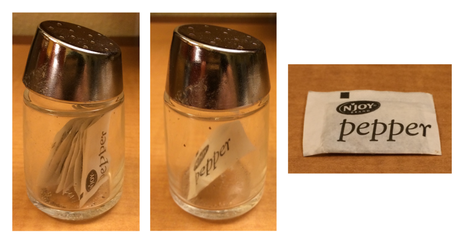
pepper[1]. (Right) pepper[[1]]
This same principle applies when you use 1d [ with a data frame: df["x"] returns a one-column data frame and df[["x"]] returns a vector.
当你对数据框使用一维 [ 时,同样的原则也适用:df["x"] 返回一个单列数据框,而 df[["x"]] 返回一个向量。
27.3.4 Exercises
What happens when you use
[[with a positive integer that’s bigger than the length of the vector? What happens when you subset with a name that doesn’t exist?What would
pepper[[1]][1]be? What aboutpepper[[1]][[1]]?
27.4 Apply family
In Chapter 26, you learned tidyverse techniques for iteration like dplyr::across() and the map family of functions. In this section, you’ll learn about their base equivalents, the apply family. In this context apply and map are synonyms because another way of saying “map a function over each element of a vector” is “apply a function over each element of a vector”. Here we’ll give you a quick overview of this family so you can recognize them in the wild.
在 Chapter 26 中,你学习了 tidyverse 的迭代技术,如 dplyr::across() 和 map 系列函数。在本节中,你将学习它们在基础 R 中的等价物,即 apply 家族。在这种情况下,apply 和 map 是同义词,因为“将函数映射到向量的每个元素上”的另一种说法是“将函数应用于向量的每个元素上”。这里我们将快速介绍这个家族,以便你在实际中能认出它们。
The most important member of this family is lapply(), which is very similar to purrr::map()3. In fact, because we haven’t used any of map()’s more advanced features, you can replace every map() call in Chapter 26 with lapply().
这个家族中最重要的成员是 lapply(),它与 purrr::map() 非常相似3。事实上,因为我们没有使用 map() 的任何更高级的功能,你可以用 lapply() 替换 Chapter 26 中的每一个 map() 调用。
There’s no exact base R equivalent to across() but you can get close by using [ with lapply(). This works because under the hood, data frames are lists of columns, so calling lapply() on a data frame applies the function to each column.
基础 R 中没有与 across() 完全等价的函数,但你可以通过将 [ 与 lapply() 结合使用来接近它的功能。这样做是可行的,因为在底层,数据框是列的列表,所以对数据框调用 lapply() 会将函数应用于每一列。
df <- tibble(a = 1, b = 2, c = "a", d = "b", e = 4)

# First find numeric columns
num_cols <- sapply(df, is.numeric)
num_cols
#>     a     b     c     d     e
#>  TRUE  TRUE FALSE FALSE  TRUE

# Then transform each column with lapply() then replace the original values
df[, num_cols] <- lapply(df[, num_cols, drop = FALSE], \(x) x * 2)
df
#> # A tibble: 1 × 5
#>       a     b c     d         e
#>   <dbl> <dbl> <chr> <chr> <dbl>
#> 1     2     4 a     b         8
The code above uses a new function, sapply(). It’s similar to lapply() but it always tries to simplify the result, hence the s in its name, here producing a logical vector instead of a list. We don’t recommend using it for programming, because the simplification can fail and give you an unexpected type, but it’s usually fine for interactive use. purrr has a similar function called map_vec() that we didn’t mention in Chapter 26.
上面的代码使用了一个新函数 sapply()。它与 lapply() 相似,但它总是尝试简化结果,因此其名称中带有 s,这里它产生一个逻辑向量而不是一个列表。我们不建议在编程中使用它,因为简化可能会失败并给你一个意想不到的类型,但对于交互式使用来说通常没问题。purrr 有一个类似的函数叫做 map_vec(),我们在 Chapter 26 中没有提到。
Base R provides a stricter version of sapply() called vapply(), short for vector apply. It takes an additional argument that specifies the expected type, ensuring that simplification occurs the same way regardless of the input. For example, we could replace the sapply() call above with this vapply() where we specify that we expect is.numeric() to return a logical vector of length 1:
基础 R 提供了一个更严格的 sapply() 版本,名为 vapply(),是 vector apply 的缩写。它接受一个额外的参数来指定预期的类型,确保无论输入如何,简化都以相同的方式发生。例如,我们可以用这个 vapply() 替换上面的 sapply() 调用,我们在其中指定我们期望 is.numeric() 返回一个长度为 1 的逻辑向量:
The distinction between sapply() and vapply() is really important when they’re inside a function (because it makes a big difference to the function’s robustness to unusual inputs), but it doesn’t usually matter in data analysis.sapply() 和 vapply() 之间的区别在它们位于函数内部时非常重要(因为它对函数对异常输入的鲁棒性有很大影响),但在数据分析中通常无关紧要。
Another important member of the apply family is tapply() which computes a single grouped summary:
apply 家族的另一个重要成员是 tapply(),它计算单个分组摘要:
diamonds |>
  group_by(cut) |>
  summarize(price = mean(price))
#> # A tibble: 5 × 2
#>   cut       price
#>   <ord>     <dbl>
#> 1 Fair      4359.
#> 2 Good      3929.
#> 3 Very Good 3982.
#> 4 Premium   4584.
#> 5 Ideal     3458.

tapply(diamonds$price, diamonds$cut, mean)
#>      Fair      Good Very Good   Premium     Ideal
#>  4358.758  3928.864  3981.760  4584.258  3457.542
Unfortunately tapply() returns its results in a named vector which requires some gymnastics if you want to collect multiple summaries and grouping variables into a data frame (it’s certainly possible to not do this and just work with free floating vectors, but in our experience that just delays the work). If you want to see how you might use tapply() or other base techniques to perform other grouped summaries, Hadley has collected a few techniques in a gist.
不幸的是,tapply() 以命名向量的形式返回其结果,如果你想将多个摘要和分组变量收集到一个数据框中,就需要一些技巧(当然可以不这样做,只使用自由浮动的向量,但根据我们的经验,这只是推迟了工作)。如果你想看看如何使用 tapply() 或其他基础技术来执行其他分组摘要,Hadley 在 一个 gist 中收集了一些技巧。
The final member of the apply family is the titular apply(), which works with matrices and arrays. In particular, watch out for apply(df, 2, something), which is a slow and potentially dangerous way of doing lapply(df, something). This rarely comes up in data science because we usually work with data frames and not matrices.
apply 家族的最后一个成员是同名的 apply(),它用于处理矩阵和数组。特别要注意 apply(df, 2, something),这是一种缓慢且可能危险的方式来执行 lapply(df, something)。这在数据科学中很少出现,因为我们通常处理数据框而不是矩阵。
27.5 for loops
for loops are the fundamental building block of iteration that both the apply and map families use under the hood. for loops are powerful and general tools that are important to learn as you become a more experienced R programmer. The basic structure of a for loop looks like this:for 循环是迭代的基本构建块,apply 和 map 家族在底层都使用了它。for 循环是强大而通用的工具,随着你成为一名更有经验的 R 程序员,学习它们非常重要。for 循环的基本结构如下:
for (element in vector) {
  # do something with element
}
The most straightforward use of for loops is to achieve the same effect as walk(): call some function with a side-effect on each element of a list. For example, in Section 26.4.1 instead of using walk():for 循环最直接的用途是实现与 walk() 相同的效果:对列表的每个元素调用某个具有副作用的函数。例如,在 Section 26.4.1 中,我们可以不使用 walk():
paths |> walk(append_file)We could have used a for loop:
而是使用 for 循环:
for (path in paths) {
  append_file(path)
}
Things get a little trickier if you want to save the output of the for loop, for example reading all of the excel files in a directory like we did in Chapter 26:
如果你想保存 for 循环的输出,事情会变得稍微复杂一些,例如,像我们在 Chapter 26 中所做的那样,读取目录中所有的 excel 文件:
paths <- dir("data/gapminder", pattern = "\\.xlsx$", full.names = TRUE)
files <- map(paths, readxl::read_excel)
There are a few different techniques that you can use, but we recommend being explicit about what the output is going to look like upfront. In this case, we’re going to want a list the same length as paths, which we can create with vector():
你可以使用几种不同的技术,但我们建议预先明确输出的样子。在这种情况下,我们需要一个与 paths 长度相同的列表,我们可以用 vector() 创建它:
Then instead of iterating over the elements of paths, we’ll iterate over their indices, using seq_along() to generate one index for each element of paths:
然后,我们不遍历 paths 的元素,而是遍历它们的索引,使用 seq_along() 为 paths 的每个元素生成一个索引:
seq_along(paths)
#>  [1]  1  2  3  4  5  6  7  8  9 10 11 12
Using the indices is important because it allows us to link to each position in the input with the corresponding position in the output:
使用索引很重要,因为它允许我们将输入中的每个位置与输出中相应的位置链接起来:
for (i in seq_along(paths)) {
  files[[i]] <- readxl::read_excel(paths[[i]])
}
To combine the list of tibbles into a single tibble you can use do.call() + rbind():
要将 tibble 列表合并为单个 tibble,你可以使用 do.call() + rbind():
do.call(rbind, files)
#> # A tibble: 1,704 × 5
#>   country     continent lifeExp      pop gdpPercap
#>   <chr>       <chr>       <dbl>    <dbl>     <dbl>
#> 1 Afghanistan Asia         28.8  8425333      779.
#> 2 Albania     Europe       55.2  1282697     1601.
#> 3 Algeria     Africa       43.1  9279525     2449.
#> 4 Angola      Africa       30.0  4232095     3521.
#> 5 Argentina   Americas     62.5 17876956     5911.
#> 6 Australia   Oceania      69.1  8691212    10040.
#> # ℹ 1,698 more rows
Rather than making a list and saving the results as we go, a simpler approach is to build up the data frame piece-by-piece:
与其创建一个列表并随时保存结果,一个更简单的方法是逐个构建数据框:
out <- NULL
for (path in paths) {
  out <- rbind(out, readxl::read_excel(path))
}
We recommend avoiding this pattern because it can become very slow when the vector is very long. This is the source of the persistent canard that for loops are slow: they’re not, but iteratively growing a vector is.
我们建议避免这种模式,因为当向量非常长时,它会变得非常慢。这就是 for 循环很慢这个谣言的来源:它们本身不慢,但迭代地增长一个向量是慢的。
27.6 Plots
Many R users who don’t otherwise use the tidyverse prefer ggplot2 for plotting due to helpful features like sensible defaults, automatic legends, and a modern look. However, base R plotting functions can still be useful because they’re so concise — it takes very little typing to do a basic exploratory plot.
许多不使用 tidyverse 的 R 用户也喜欢用 ggplot2 来绘图,因为它有许多有用的功能,比如合理的默认设置、自动图例和现代的外观。然而,基础 R 的绘图函数仍然很有用,因为它们非常简洁——做一个基本的探索性图表只需要很少的输入。
There are two main types of base plot you’ll see in the wild: scatterplots and histograms, produced with plot() and hist() respectively. Here’s a quick example from the diamonds dataset:
你在实践中会看到两种主要的基础图类型:散点图和直方图,分别用 plot() 和 hist() 生成。这里有一个来自 diamonds 数据集的快速示例:
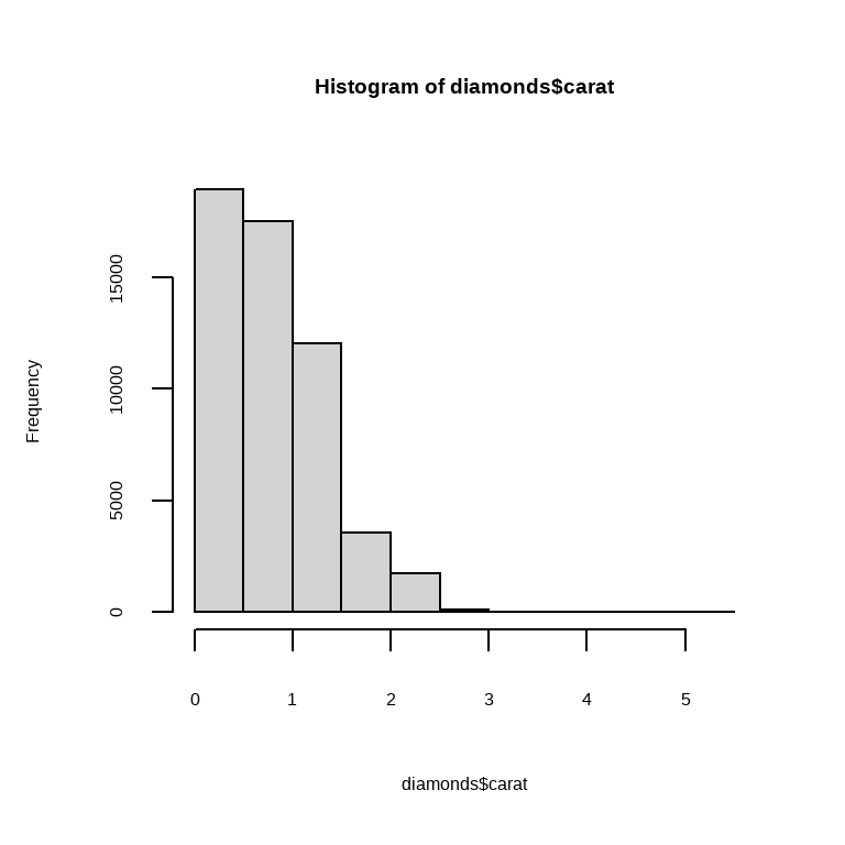
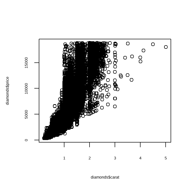
Note that base plotting functions work with vectors, so you need to pull columns out of the data frame using $ or some other technique.
请注意,基础绘图函数是作用于向量的,所以你需要使用 $ 或其他技术从数据框中提取列。
27.7 Summary
In this chapter, we’ve shown you a selection of base R functions useful for subsetting and iteration. Compared to approaches discussed elsewhere in the book, these functions tend to have more of a “vector” flavor than a “data frame” flavor because base R functions tend to take individual vectors, rather than a data frame and some column specification. This often makes life easier for programming and so becomes more important as you write more functions and begin to write your own packages.
在本章中,我们向你展示了一些用于子集和迭代的基础 R 函数。与本书其他地方讨论的方法相比,这些函数更具“向量”风格而非“数据框”风格,因为基础 R 函数倾向于接受单个向量,而不是数据框和一些列规范。这通常使编程生活更轻松,因此在你编写更多函数并开始编写自己的包时变得更加重要。
This chapter concludes the programming section of the book. You’ve made a solid start on your journey to becoming not just a data scientist who uses R, but a data scientist who can program in R. We hope these chapters have sparked your interest in programming and that you’re looking forward to learning more outside of this book.
本章结束了本书的编程部分。你已经在成为一名不仅使用 R 的数据科学家,而且是能够用 R 编程 的数据科学家的道路上迈出了坚实的一步。我们希望这些章节能激发你对编程的兴趣,并期待你在本书之外学习更多内容。
Read https://adv-r.hadley.nz/subsetting.html#subset-multiple to see how you can also subset a data frame like it is a 1d object and how you can subset it with a matrix.↩︎
But it doesn’t handle grouped data frames differently and it doesn’t support selection helper functions like
starts_with().↩︎It just lacks convenient features like progress bars and reporting which element caused the problem if there’s an error.↩︎