11 Communication

11.1 Introduction

In Chapter 10, you learned how to use plots as tools for exploration. When you make exploratory plots, you know—even before looking—which variables the plot will display. You made each plot for a purpose, could quickly look at it, and then move on to the next plot. In the course of most analyses, you’ll produce tens or hundreds of plots, most of which are immediately thrown away.
在 Chapter 10 中，你学习了如何使用图形作为探索的工具。当你制作探索性图形时，你甚至在看图之前就知道它将显示哪些变量。你制作的每个图形都有其目的，可以快速浏览一下，然后继续制作下一个。在大多数分析过程中，你会生成数十甚至数百个图形，其中大部分都会被立即丢弃。

Now that you understand your data, you need to communicate your understanding to others. Your audience will likely not share your background knowledge and will not be deeply invested in the data. To help others quickly build up a good mental model of the data, you will need to invest considerable effort in making your plots as self-explanatory as possible. In this chapter, you’ll learn some of the tools that ggplot2 provides to do so.
现在你已经理解了你的数据，你需要将你的理解传达给他人。你的受众很可能不具备你的背景知识，也不会对数据投入太多精力。为了帮助他人快速建立起对数据的良好心智模型，你需要投入大量精力使你的图形尽可能地不言自明。在本章中，你将学习 ggplot2 为此提供的一些工具。

This chapter focuses on the tools you need to create good graphics. We assume that you know what you want, and just need to know how to do it. For that reason, we highly recommend pairing this chapter with a good general visualization book. We particularly like The Truthful Art, by Albert Cairo. It doesn’t teach the mechanics of creating visualizations, but instead focuses on what you need to think about in order to create effective graphics.
本章重点介绍创建优秀图形所需的工具。我们假设你已经知道自己想要什么，只需要知道如何实现它。因此，我们强烈建议将本章与一本优秀的通用可视化书籍结合阅读。我们特别推荐 Albert Cairo 的 The Truthful Art。这本书不教你创建可视化的具体操作，而是专注于为了创作有效的图形你需要思考些什么。

11.1.1 Prerequisites

In this chapter, we’ll focus once again on ggplot2. We’ll also use a little dplyr for data manipulation, scales to override the default breaks, labels, transformations and palettes, and a few ggplot2 extension packages, including ggrepel (https://ggrepel.slowkow.com) by Kamil Slowikowski and patchwork (https://patchwork.data-imaginist.com) by Thomas Lin Pedersen. Don’t forget that you’ll need to install those packages with install.packages() if you don’t already have them.
在本章中，我们将再次聚焦于 ggplot2。我们还会使用一些 dplyr 进行数据操作，使用 scales 包来覆盖默认的刻度、标签、变换和调色板，以及一些 ggplot2 扩展包，包括 Kamil Slowikowski 开发的 ggrepel (https://ggrepel.slowkow.com) 和 Thomas Lin Pedersen 开发的 patchwork (https://patchwork.data-imaginist.com)。如果你还没有安装这些包，别忘了用 install.packages() 来安装它们。

library(tidyverse)
library(scales)
library(ggrepel)
library(patchwork)

11.2 Labels

The easiest place to start when turning an exploratory graphic into an expository graphic is with good labels. You add labels with the labs() function.
将探索性图形转变为解释性图形，最简单的入手点就是添加良好的标签。你可以使用 labs() 函数来添加标签。

ggplot(mpg, aes(x = displ, y = hwy)) +
  geom_point(aes(color = class)) +
  geom_smooth(se = FALSE) +
  labs(
    x = "Engine displacement (L)",
    y = "Highway fuel economy (mpg)",
    color = "Car type",
    title = "Fuel efficiency generally decreases with engine size",
    subtitle = "Two seaters (sports cars) are an exception because of their light weight",
    caption = "Data from fueleconomy.gov"
  )

Scatterplot of highway fuel efficiency versus engine size of cars, where points are colored according to the car class. A smooth curve following the trajectory of the relationship between highway fuel efficiency versus engine size of cars is overlaid. The x-axis is labelled "Engine displacement (L)" and the y-axis is labelled "Highway fuel economy (mpg)". The legend is labelled "Car type". The plot is titled "Fuel efficiency generally decreases with engine size". The subtitle is "Two seaters (sports cars) are an exception because of their light weight" and the caption is "Data from fueleconomy.gov".

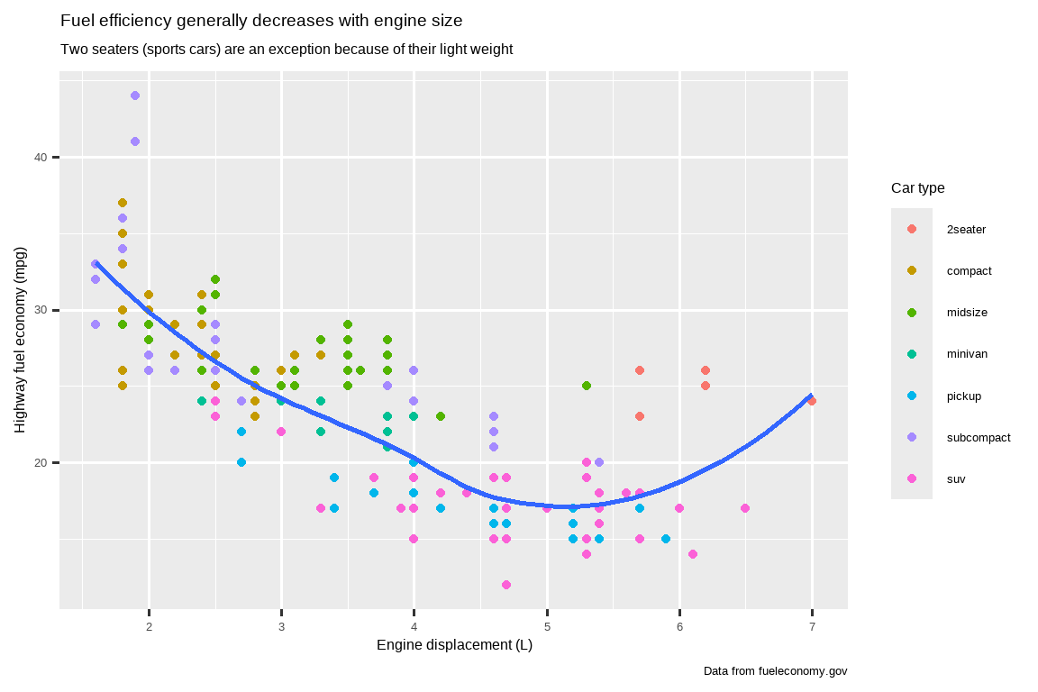
The purpose of a plot title is to summarize the main finding. Avoid titles that just describe what the plot is, e.g., “A scatterplot of engine displacement vs. fuel economy”.
图形标题的目的是总结主要发现。应避免使用仅仅描述图形内容的标题，例如“发动机排量与燃油经济性的散点图”。

If you need to add more text, there are two other useful labels: subtitle adds additional detail in a smaller font beneath the title and caption adds text at the bottom right of the plot, often used to describe the source of the data. You can also use labs() to replace the axis and legend titles. It’s usually a good idea to replace short variable names with more detailed descriptions, and to include the units.
如果你需要添加更多文字，还有两个有用的标签：subtitle (副标题) 会在主标题下方以较小字体添加额外细节，而 caption (说明文字) 会在图形右下角添加文字，通常用来描述数据来源。你也可以使用 labs() 来替换坐标轴和图例的标题。通常，用更详细的描述替换简短的变量名，并包含单位，是一个好主意。

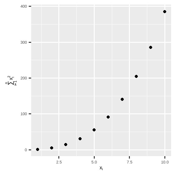
It’s possible to use mathematical equations instead of text strings. Just switch "" out for quote() and read about the available options in ?plotmath:
你也可以使用数学公式代替文本字符串。只需将 "" 换成 quote()，并在 ?plotmath 中阅读有关可用选项的信息：

df <- tibble(
  x = 1:10,
  y = cumsum(x^2)
)

ggplot(df, aes(x, y)) +
  geom_point() +
  labs(
    x = quote(x[i]),
    y = quote(sum(x[i] ^ 2, i == 1, n))
  )

Scatterplot with math text on the x and y axis labels. X-axis label says x_i, y-axis label says sum of x_i squared, for i from 1 to n.

11.2.1 Exercises

Create one plot on the fuel economy data with customized title, subtitle, caption, x, y, and color labels.
Recreate the following plot using the fuel economy data. Note that both the colors and shapes of points vary by type of drive train.
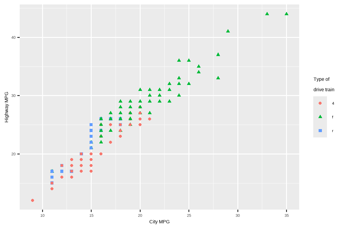
Take an exploratory graphic that you’ve created in the last month, and add informative titles to make it easier for others to understand.

11.3 Annotations

In addition to labelling major components of your plot, it’s often useful to label individual observations or groups of observations. The first tool you have at your disposal is geom_text(). geom_text() is similar to geom_point(), but it has an additional aesthetic: label. This makes it possible to add textual labels to your plots.
除了为图形的主要组件添加标签外，为单个观测或观测组添加标签也常常很有用。你可以使用的第一个工具是 geom_text()。geom_text() 类似于 geom_point()，但它有一个额外的美学属性：label。这使得你可以在图形中添加文本标签。

There are two possible sources of labels. First, you might have a tibble that provides labels. In the following plot we pull out the cars with the highest engine size in each drive type and save their information as a new data frame called label_info.
标签有两个可能的来源。首先，你可能有一个提供标签的 tibble。在下面的图形中，我们提取了每种驱动类型中发动机尺寸最大的汽车，并将其信息保存为一个名为 label_info 的新数据框。

label_info <- mpg |>
  group_by(drv) |>
  arrange(desc(displ)) |>
  slice_head(n = 1) |>
  mutate(
    drive_type = case_when(
      drv == "f" ~ "front-wheel drive",
      drv == "r" ~ "rear-wheel drive",
      drv == "4" ~ "4-wheel drive"
    )
  ) |>
  select(displ, hwy, drv, drive_type)

label_info
#> # A tibble: 3 × 4
#> # Groups:   drv [3]
#>   displ   hwy drv   drive_type       
#>   <dbl> <int> <chr> <chr>            
#> 1   6.5    17 4     4-wheel drive    
#> 2   5.3    25 f     front-wheel drive
#> 3   7      24 r     rear-wheel drive

Then, we use this new data frame to directly label the three groups to replace the legend with labels placed directly on the plot. Using the fontface and size arguments we can customize the look of the text labels. They’re larger than the rest of the text on the plot and bolded. (theme(legend.position = "none") turns all the legends off — we’ll talk about it more shortly.)
然后，我们使用这个新的数据框来直接标记这三个组，用直接放置在图上的标签取代图例。通过使用 fontface 和 size 参数，我们可以自定义文本标签的外观。它们比图上其他文本更大并且加粗了。(theme(legend.position = "none") 会关闭所有图例——我们稍后会更详细地讨论它。)

ggplot(mpg, aes(x = displ, y = hwy, color = drv)) +
  geom_point(alpha = 0.3) +
  geom_smooth(se = FALSE) +
  geom_text(
    data = label_info, 
    aes(x = displ, y = hwy, label = drive_type),
    fontface = "bold", size = 5, hjust = "right", vjust = "bottom"
  ) +
  theme(legend.position = "none")
#> `geom_smooth()` using method = 'loess' and formula = 'y ~ x'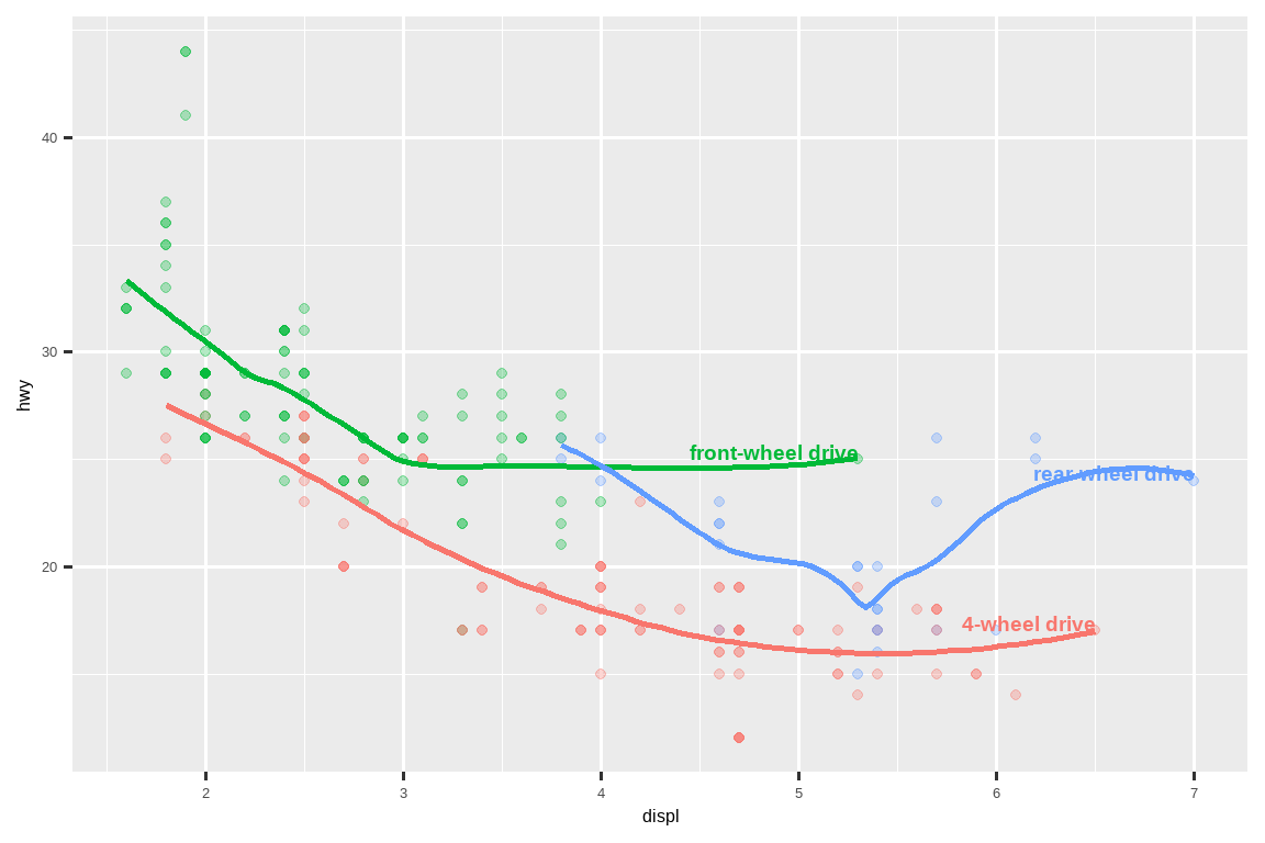

Scatterplot of highway mileage versus engine size where points are colored by drive type. Smooth curves for each drive type are overlaid. Text labels identify the curves as front-wheel, rear-wheel, and 4-wheel.

Note the use of hjust (horizontal justification) and vjust (vertical justification) to control the alignment of the label.
注意使用 hjust (水平对齐) 和 vjust (垂直对齐) 来控制标签的对齐方式。

However the annotated plot we made above is hard to read because the labels overlap with each other, and with the points. We can use the geom_label_repel() function from the ggrepel package to address both of these issues. This useful package will automatically adjust labels so that they don’t overlap:
然而，我们上面制作的带注释的图很难阅读，因为标签之间以及标签与数据点之间存在重叠。我们可以使用 ggrepel 包中的 geom_label_repel() 函数来解决这两个问题。这个有用的包会自动调整标签，使其不重叠：

ggplot(mpg, aes(x = displ, y = hwy, color = drv)) +
  geom_point(alpha = 0.3) +
  geom_smooth(se = FALSE) +
  geom_label_repel(
    data = label_info, 
    aes(x = displ, y = hwy, label = drive_type),
    fontface = "bold", size = 5, nudge_y = 2
  ) +
  theme(legend.position = "none")
#> `geom_smooth()` using method = 'loess' and formula = 'y ~ x'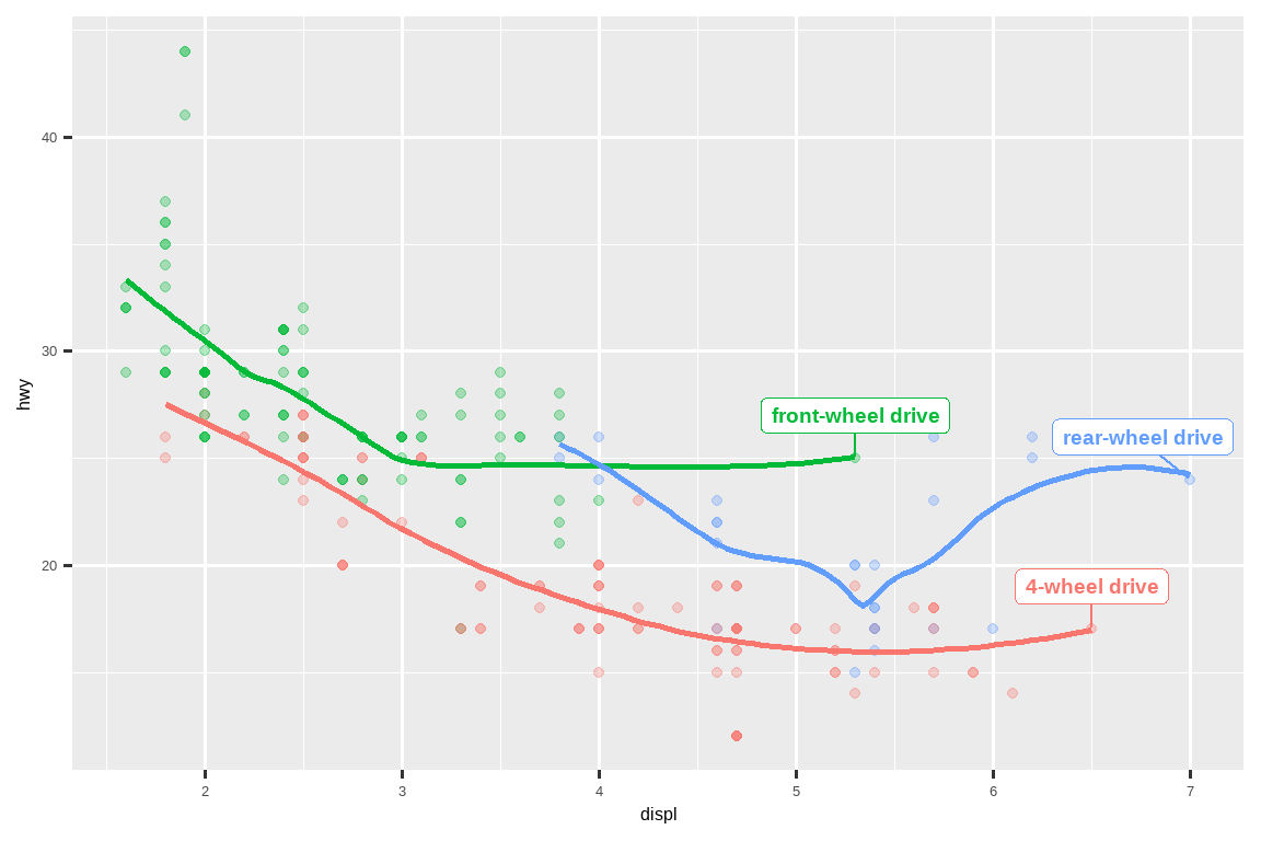

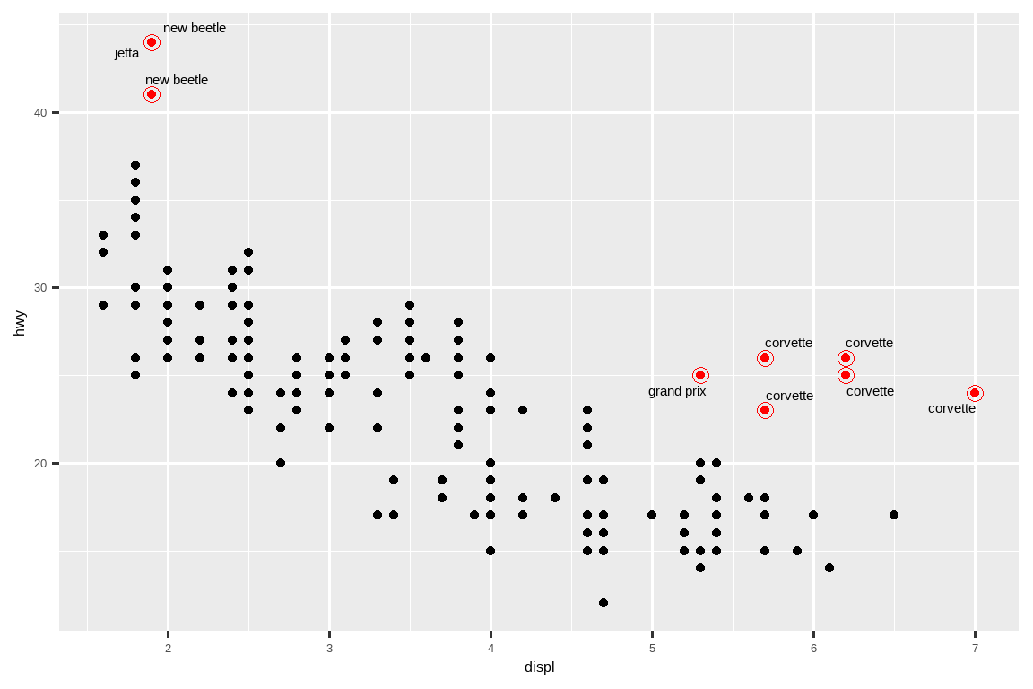
You can also use the same idea to highlight certain points on a plot with geom_text_repel() from the ggrepel package. Note another handy technique used here: we added a second layer of large, hollow points to further highlight the labelled points.
你也可以用同样的方法，使用 ggrepel 包中的 geom_text_repel() 来高亮图上的某些点。注意这里使用的另一个便捷技巧：我们添加了第二层大的空心点，以进一步突出显示被标记的点。

potential_outliers <- mpg |>
  filter(hwy > 40 | (hwy > 20 & displ > 5))
  
ggplot(mpg, aes(x = displ, y = hwy)) +
  geom_point() +
  geom_text_repel(data = potential_outliers, aes(label = model)) +
  geom_point(data = potential_outliers, color = "red") +
  geom_point(
    data = potential_outliers,
    color = "red", size = 3, shape = "circle open"
  )

Scatterplot of highway fuel efficiency versus engine size of cars. Points where highway mileage is above 40 as well as above 20 with engine size above 5 are red, with a hollow red circle, and labelled with model name of the car.

Remember, in addition to geom_text() and geom_label(), you have many other geoms in ggplot2 available to help annotate your plot. A couple ideas:
请记住，除了 geom_text() 和 geom_label() 之外，ggplot2 中还有许多其他几何对象 (geom) 可以帮助你注释图形。有几个想法：

Use geom_hline() and geom_vline() to add reference lines. We often make them thick (linewidth = 2) and white (color = white), and draw them underneath the primary data layer. That makes them easy to see, without drawing attention away from the data.
我们通常将它们设置得较粗 (linewidth = 2) 且为白色 (color = white)，并将其绘制在主数据层的下方。<br>这样既容易看到，又不会分散对数据的注意力。
Use geom_rect() to draw a rectangle around points of interest. The boundaries of the rectangle are defined by aesthetics xmin, xmax, ymin, ymax. Alternatively, look into the ggforce package, specifically geom_mark_hull(), which allows you to annotate subsets of points with hulls.
矩形的边界由美学属性 xmin、xmax、ymin、ymax 定义。<br>或者，可以研究一下 ggforce 包，特别是 geom_mark_hull()，它允许你用凸包来注释点的子集。
Use geom_segment() with the arrow argument to draw attention to a point with an arrow. Use aesthetics x and y to define the starting location, and xend and yend to define the end location.
使用美学属性 x 和 y 定义起始位置，xend 和 yend 定义结束位置。

Another handy function for adding annotations to plots is annotate(). As a rule of thumb, geoms are generally useful for highlighting a subset of the data while annotate() is useful for adding one or few annotation elements to a plot.
另一个为图形添加注释的便捷函数是 annotate()。根据经验，几何对象 (geom) 通常用于高亮显示数据的子集，而 annotate() 则适用于向图形中添加一个或几个注释元素。

To demonstrate using annotate(), let’s create some text to add to our plot. The text is a bit long, so we’ll use stringr::str_wrap() to automatically add line breaks to it given the number of characters you want per line:
为了演示 annotate() 的用法，让我们创建一些文本添加到图中。这段文本有点长，所以我们使用 stringr::str_wrap()，根据你希望每行显示的字符数来自动为其添加换行符：

trend_text <- "Larger engine sizes tend to have lower fuel economy." |>
  str_wrap(width = 30)
trend_text
#> [1] "Larger engine sizes tend to\nhave lower fuel economy."

Then, we add two layers of annotation: one with a label geom and the other with a segment geom. The x and y aesthetics in both define where the annotation should start, and the xend and yend aesthetics in the segment annotation define the end location of the segment. Note also that the segment is styled as an arrow.
然后，我们添加两层注释：一层是标签几何对象，另一层是线段几何对象。两者中的 x 和 y 美学属性定义了注释的起始位置，而线段注释中的 xend 和 yend 美学属性定义了线段的结束位置。还要注意，该线段被样式化为箭头。

ggplot(mpg, aes(x = displ, y = hwy)) +
  geom_point() +
  annotate(
    geom = "label", x = 3.5, y = 38,
    label = trend_text,
    hjust = "left", color = "red"
  ) +
  annotate(
    geom = "segment",
    x = 3, y = 35, xend = 5, yend = 25, color = "red",
    arrow = arrow(type = "closed")
  )

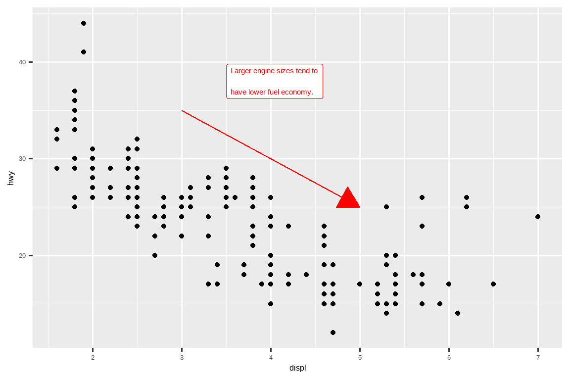
Scatterplot of highway fuel efficiency versus engine size of cars. A red arrow pointing down follows the trend of the points and the annotation placed next to the arrow reads "Larger engine sizes tend to have lower fuel economy". The arrow and the annotation text is red.

Annotation is a powerful tool for communicating main takeaways and interesting features of your visualizations. The only limit is your imagination (and your patience with positioning annotations to be aesthetically pleasing)!
注释是传达可视化主要结论和有趣特征的强大工具。唯一的限制是你的想象力（以及你为美观地定位注释而付出的耐心）！

11.3.1 Exercises

Use geom_text() with infinite positions to place text at the four corners of the plot.
Use annotate() to add a point geom in the middle of your last plot without having to create a tibble. Customize the shape, size, or color of the point.
How do labels with geom_text() interact with faceting? How can you add a label to a single facet? How can you put a different label in each facet? (Hint: Think about the dataset that is being passed to geom_text().)
What arguments to geom_label() control the appearance of the background box?
What are the four arguments to arrow()? How do they work? Create a series of plots that demonstrate the most important options.

11.4 Scales

The third way you can make your plot better for communication is to adjust the scales. Scales control how the aesthetic mappings manifest visually.
让你的图表更易于交流的第三种方法是调整标度（scales）。标度控制着美学映射（aesthetic mappings）在视觉上的表现方式。

11.4.1 Default scales

Normally, ggplot2 automatically adds scales for you. For example, when you type:
通常情况下，ggplot2 会自动为你添加标度。例如，当你输入：

ggplot(mpg, aes(x = displ, y = hwy)) +
  geom_point(aes(color = class))

ggplot2 automatically adds default scales behind the scenes:
ggplot2 会在后台自动添加默认的标度：

ggplot(mpg, aes(x = displ, y = hwy)) +
  geom_point(aes(color = class)) +
  scale_x_continuous() +
  scale_y_continuous() +
  scale_color_discrete()

Note the naming scheme for scales: scale_ followed by the name of the aesthetic, then _, then the name of the scale. The default scales are named according to the type of variable they align with: continuous, discrete, datetime, or date. scale_x_continuous() puts the numeric values from displ on a continuous number line on the x-axis, scale_color_discrete() chooses colors for each of the class of car, etc. There are lots of non-default scales which you’ll learn about below.
注意标度的命名方案：scale_ 后跟美学属性的名称，然后是 _，再后跟标度的名称。默认标度是根据它们所对应的变量类型来命名的：连续型 (continuous)、离散型 (discrete)、日期时间型 (datetime) 或日期型 (date)。scale_x_continuous() 将 displ 的数值放在 x 轴的连续数轴上，scale_color_discrete() 为每种汽车 class 选择颜色，等等。下面你将学习到许多非默认的标度。

The default scales have been carefully chosen to do a good job for a wide range of inputs. Nevertheless, you might want to override the defaults for two reasons:
默认标度经过精心挑选，能在各种输入下都表现良好。尽管如此，你可能出于两个原因想要覆盖默认设置：

You might want to tweak some of the parameters of the default scale. This allows you to do things like change the breaks on the axes, or the key labels on the legend.
这允许你做一些事情，比如更改坐标轴上的刻度，或图例上的键标签。
You might want to replace the scale altogether, and use a completely different algorithm. Often you can do better than the default because you know more about the data.
通常你可以做得比默认更好，因为你对数据有更多的了解。

11.4.2 Axis ticks and legend keys

Collectively axes and legends are called guides. Axes are used for x and y aesthetics; legends are used for everything else.
坐标轴和图例统称为引导元素 (guides)。坐标轴用于 x 和 y 美学属性；图例用于所有其他美学属性。

There are two primary arguments that affect the appearance of the ticks on the axes and the keys on the legend: breaks and labels. Breaks controls the position of the ticks, or the values associated with the keys. Labels controls the text label associated with each tick/key. The most common use of breaks is to override the default choice:
有两个主要参数会影响坐标轴上的刻度线和图例上的键的外观：breaks 和 labels。Breaks 控制刻度线的位置，或与键相关联的值。Labels 控制与每个刻度线/键相关联的文本标签。breaks 最常见的用途是覆盖默认选项：

ggplot(mpg, aes(x = displ, y = hwy, color = drv)) +
  geom_point() +
  scale_y_continuous(breaks = seq(15, 40, by = 5))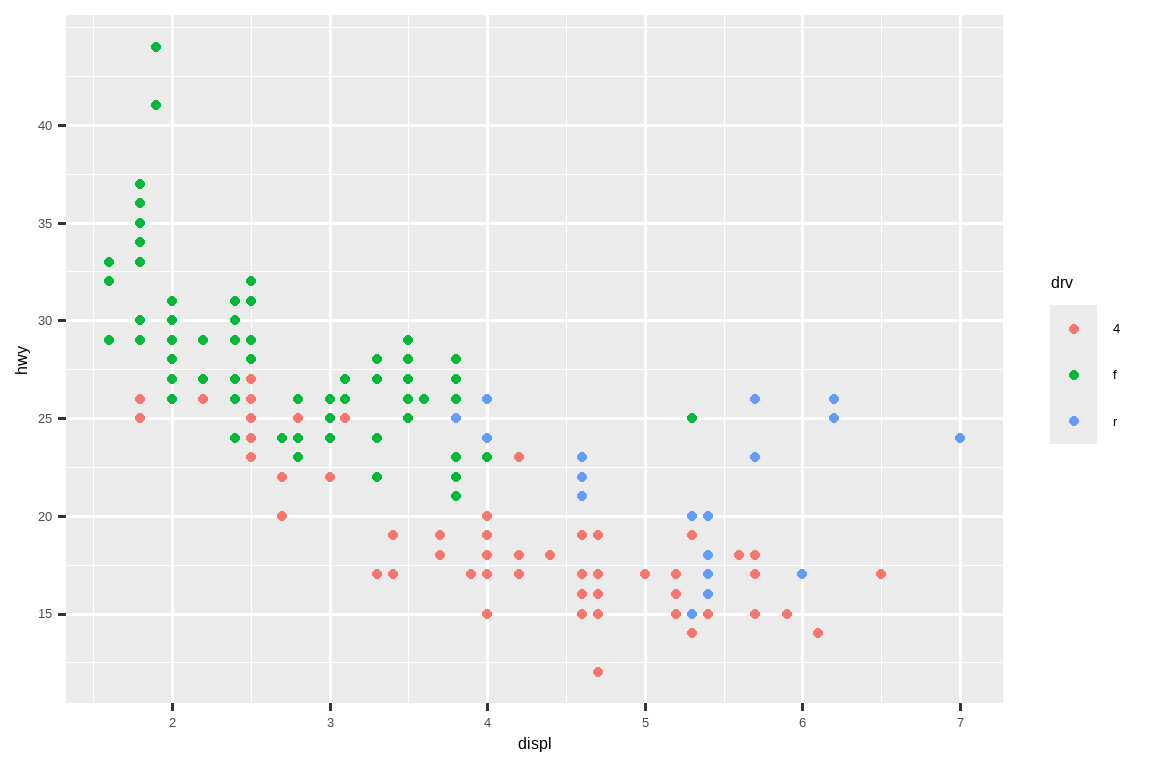

Scatterplot of highway fuel efficiency versus engine size of cars, colored by drive. The y-axis has breaks starting at 15 and ending at 40, increasing by 5.

You can use labels in the same way (a character vector the same length as breaks), but you can also set it to NULL to suppress the labels altogether. This can be useful for maps, or for publishing plots where you can’t share the absolute numbers. You can also use breaks and labels to control the appearance of legends. For discrete scales for categorical variables, labels can be a named list of the existing level names and the desired labels for them.
你可以用同样的方式使用 labels (一个与 breaks 长度相同的字符向量)，但你也可以将其设置为 NULL 来完全抑制标签。这对于地图或发布那些不能分享绝对数字的图表可能很有用。你还可以使用 breaks 和 labels 来控制图例的外观。对于分类变量的离散标度，labels 可以是一个命名列表，包含现有的水平名称和它们期望的标签。

ggplot(mpg, aes(x = displ, y = hwy, color = drv)) +
  geom_point() +
  scale_x_continuous(labels = NULL) +
  scale_y_continuous(labels = NULL) +
  scale_color_discrete(labels = c("4" = "4-wheel", "f" = "front", "r" = "rear"))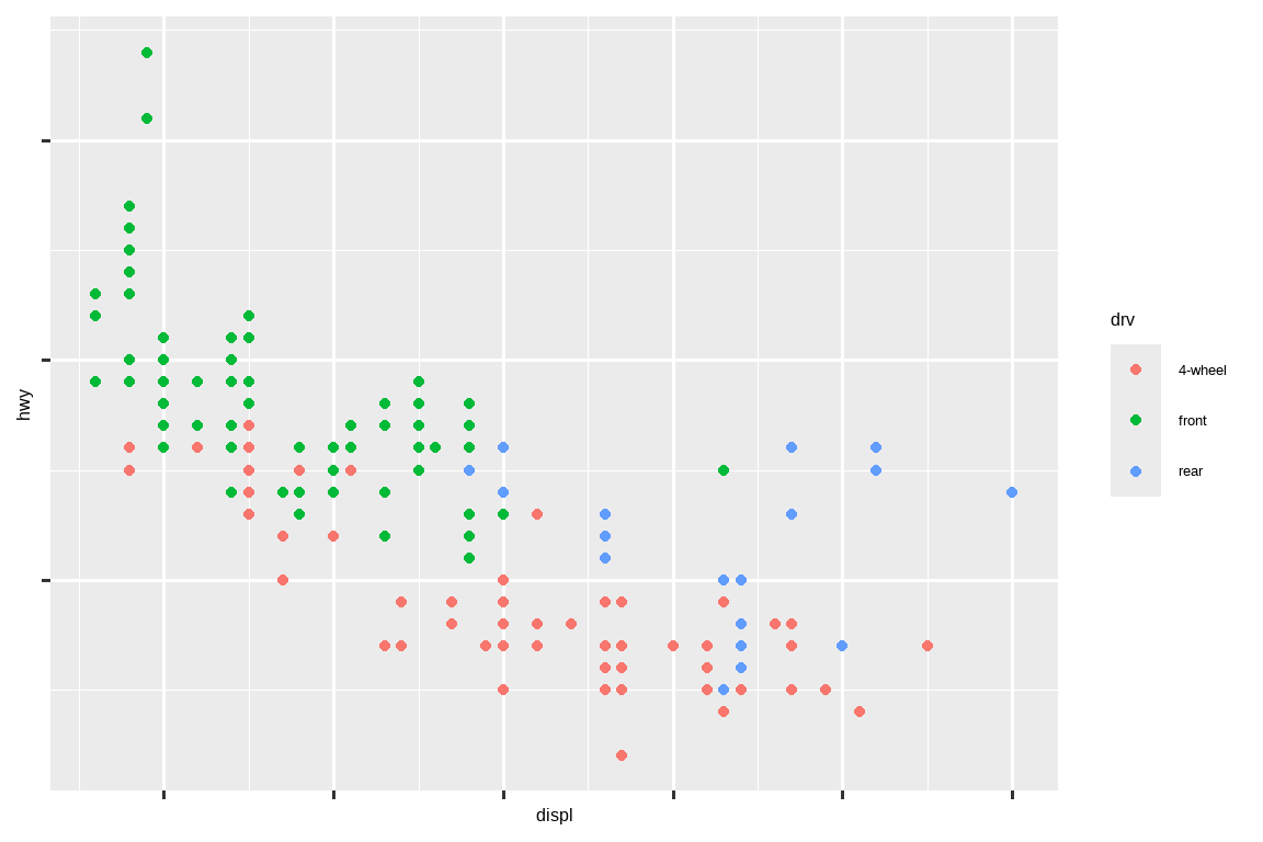

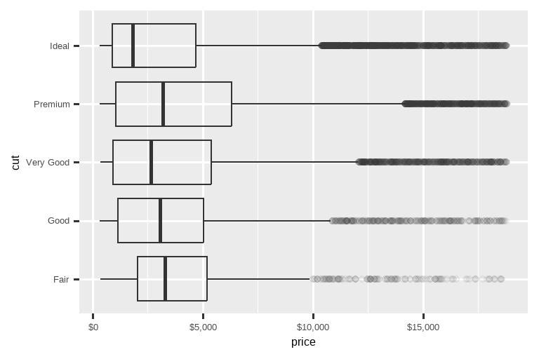
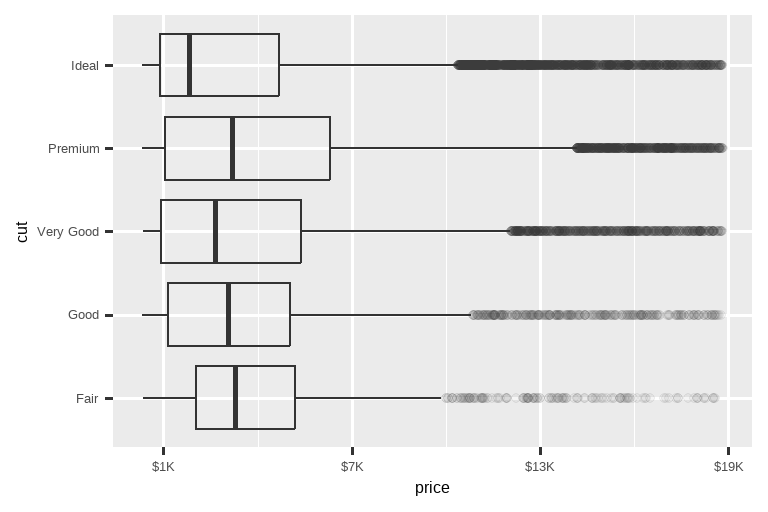
Scatterplot of highway fuel efficiency versus engine size of cars, colored by drive. The x and y-axes do not have any labels at the axis ticks. The legend has custom labels: 4-wheel, front, rear.

The labels argument coupled with labelling functions from the scales package is also useful for formatting numbers as currency, percent, etc. The plot on the left shows default labelling with label_dollar(), which adds a dollar sign as well as a thousand separator comma. The plot on the right adds further customization by dividing dollar values by 1,000 and adding a suffix “K” (for “thousands”) as well as adding custom breaks. Note that breaks is in the original scale of the data.
labels 参数与 scales 包中的标签函数相结合，对于格式化数字（如货币、百分比等）也很有用。左图展示了使用 label_dollar() 的默认标签，它会添加美元符号和千位分隔逗号。右图通过将美元值除以 1000 并添加后缀“K”（代表“千”），以及添加自定义断点，进行了进一步的定制。注意，breaks 是基于原始数据的标度。

# Left
ggplot(diamonds, aes(x = price, y = cut)) +
  geom_boxplot(alpha = 0.05) +
  scale_x_continuous(labels = label_dollar())

# Right
ggplot(diamonds, aes(x = price, y = cut)) +
  geom_boxplot(alpha = 0.05) +
  scale_x_continuous(
    labels = label_dollar(scale = 1/1000, suffix = "K"), 
    breaks = seq(1000, 19000, by = 6000)
  )

Two side-by-side box plots of price versus cut of diamonds. The outliers are transparent. On both plots the x-axis labels are formatted as dollars. The x-axis labels on the left plot start at $0 and go to $15,000, increasing by $5,000. The x-axis labels on the right plot start at $1K and go to $19K, increasing by $6K.

Another handy label function is label_percent():
另一个方便的标签函数是 label_percent()：

ggplot(diamonds, aes(x = cut, fill = clarity)) +
  geom_bar(position = "fill") +
  scale_y_continuous(name = "Percentage", labels = label_percent())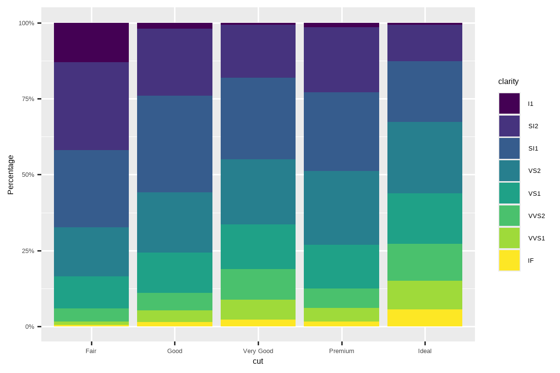

Segmented bar plots of cut, filled with levels of clarity. The y-axis labels start at 0% and go to 100%, increasing by 25%. The y-axis label name is "Percentage".

Another use of breaks is when you have relatively few data points and want to highlight exactly where the observations occur. For example, take this plot that shows when each US president started and ended their term.
breaks 的另一个用途是当你数据点相对较少，并希望精确地突出显示观测值出现的位置时。例如，看下面这张图，它显示了每位美国总统任期的起止时间。

presidential |>
  mutate(id = 33 + row_number()) |>
  ggplot(aes(x = start, y = id)) +
  geom_point() +
  geom_segment(aes(xend = end, yend = id)) +
  scale_x_date(name = NULL, breaks = presidential$start, date_labels = "'%y")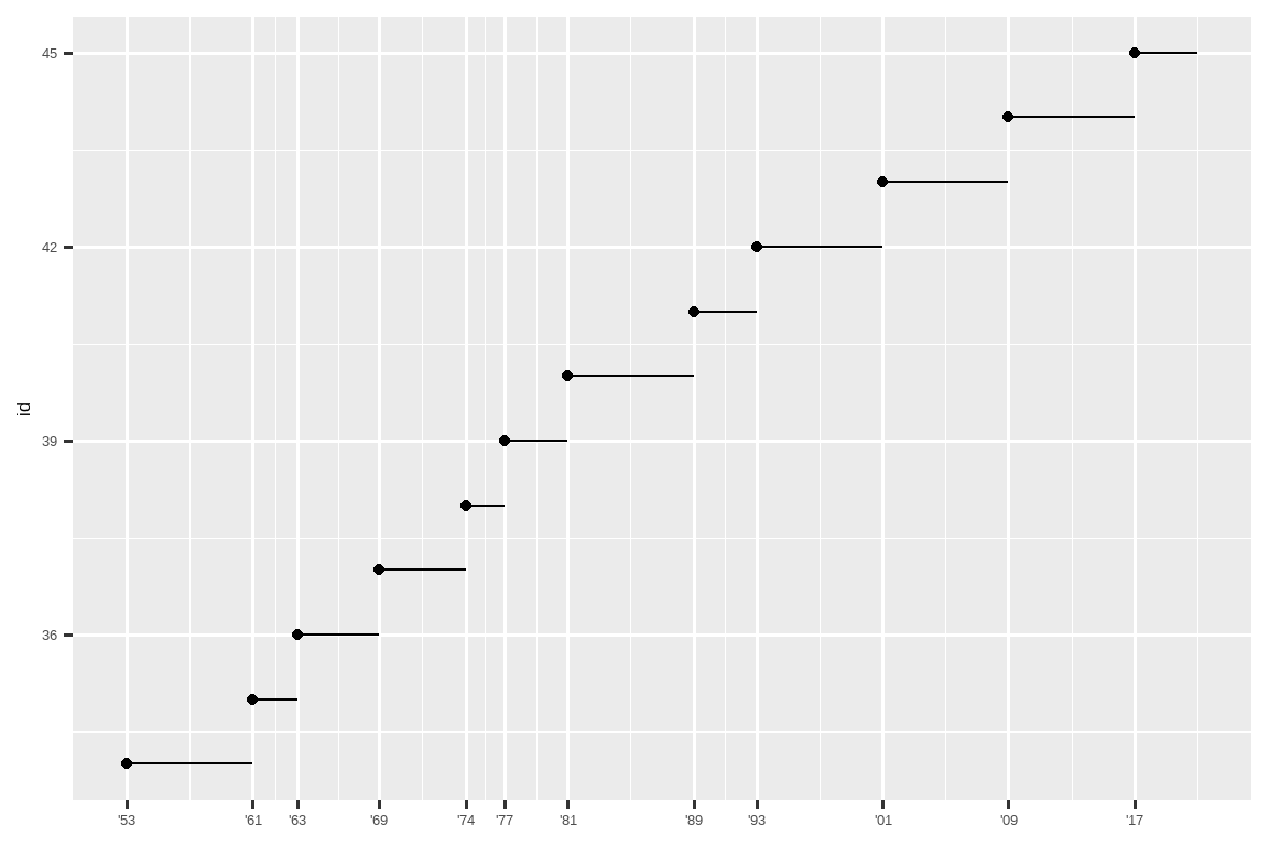

Line plot of id number of presidents versus the year they started their presidency. Start year is marked with a point and a segment that starts there and ends at the end of the presidency. The x-axis labels are formatted as two digit years starting with an apostrophe, e.g., '53.

Note that for the breaks argument we pulled out the start variable as a vector with presidential$start because we can’t do an aesthetic mapping for this argument. Also note that the specification of breaks and labels for date and datetime scales is a little different:
请注意，对于 breaks 参数，我们使用 presidential$start 将 start 变量提取为一个向量，因为我们不能对这个参数进行美学映射。另请注意，日期和日期时间标度的断点和标签的规范略有不同：

date_labels takes a format specification, in the same form as parse_datetime().
date_labels 接受一个格式规范，其形式与 parse_datetime() 相同。
date_breaks (not shown here), takes a string like “2 days” or “1 month”.
date_breaks（此处未显示）接受一个字符串，如 “2 days” 或 “1 month”。

11.4.3 Legend layout

You will most often use breaks and labels to tweak the axes. While they both also work for legends, there are a few other techniques you are more likely to use.
你最常使用 breaks 和 labels 来调整坐标轴。虽然它们也适用于图例，但你更可能使用一些其他的技巧。

To control the overall position of the legend, you need to use a theme() setting. We’ll come back to themes at the end of the chapter, but in brief, they control the non-data parts of the plot. The theme setting legend.position controls where the legend is drawn:
要控制图例的整体位置，你需要使用 theme() 设置。我们将在本章末尾再讨论主题 (themes)，但简而言之，它们控制着图表的非数据部分。主题设置 legend.position 控制图例的绘制位置：

base <- ggplot(mpg, aes(x = displ, y = hwy)) +
  geom_point(aes(color = class))

base + theme(legend.position = "right") # the default
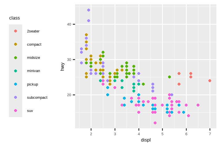
base + theme(legend.position = "left")
base + 
  theme(legend.position = "top") +
  guides(color = guide_legend(nrow = 3))
base + 
  theme(legend.position = "bottom") +
  guides(color = guide_legend(nrow = 3))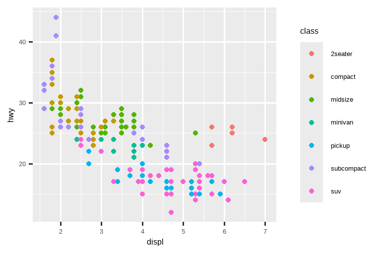

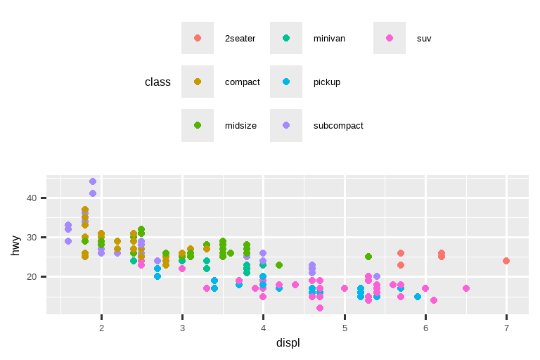
Four scatterplots of highway fuel efficiency versus engine size of cars where points are colored based on class of car. Clockwise, the legend is placed on the right, left, bottom, and top of the plot.

If your plot is short and wide, place the legend at the top or bottom, and if it’s tall and narrow, place the legend at the left or right. You can also use legend.position = "none" to suppress the display of the legend altogether.
如果你的图形又短又宽，就把图例放在顶部或底部；如果它又高又窄，就把图例放在左侧或右侧。你也可以使用 legend.position = "none" 来完全抑制图例的显示。

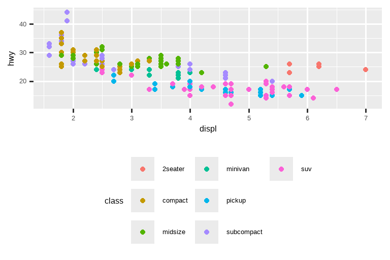
To control the display of individual legends, use guides() along with guide_legend() or guide_colorbar(). The following example shows two important settings: controlling the number of rows the legend uses with nrow, and overriding one of the aesthetics to make the points bigger. This is particularly useful if you have used a low alpha to display many points on a plot.
要控制单个图例的显示，请使用 guides() 函数，并配合 guide_legend() 或 guide_colorbar()。下面的例子展示了两个重要的设置：使用 nrow 控制图例使用的行数，以及覆盖其中一个美学属性以使点变大。如果你在图上使用了较低的 alpha 值来显示许多点，这尤其有用。

ggplot(mpg, aes(x = displ, y = hwy)) +
  geom_point(aes(color = class)) +
  geom_smooth(se = FALSE) +
  theme(legend.position = "bottom") +
  guides(color = guide_legend(nrow = 2, override.aes = list(size = 4)))
#> `geom_smooth()` using method = 'loess' and formula = 'y ~ x'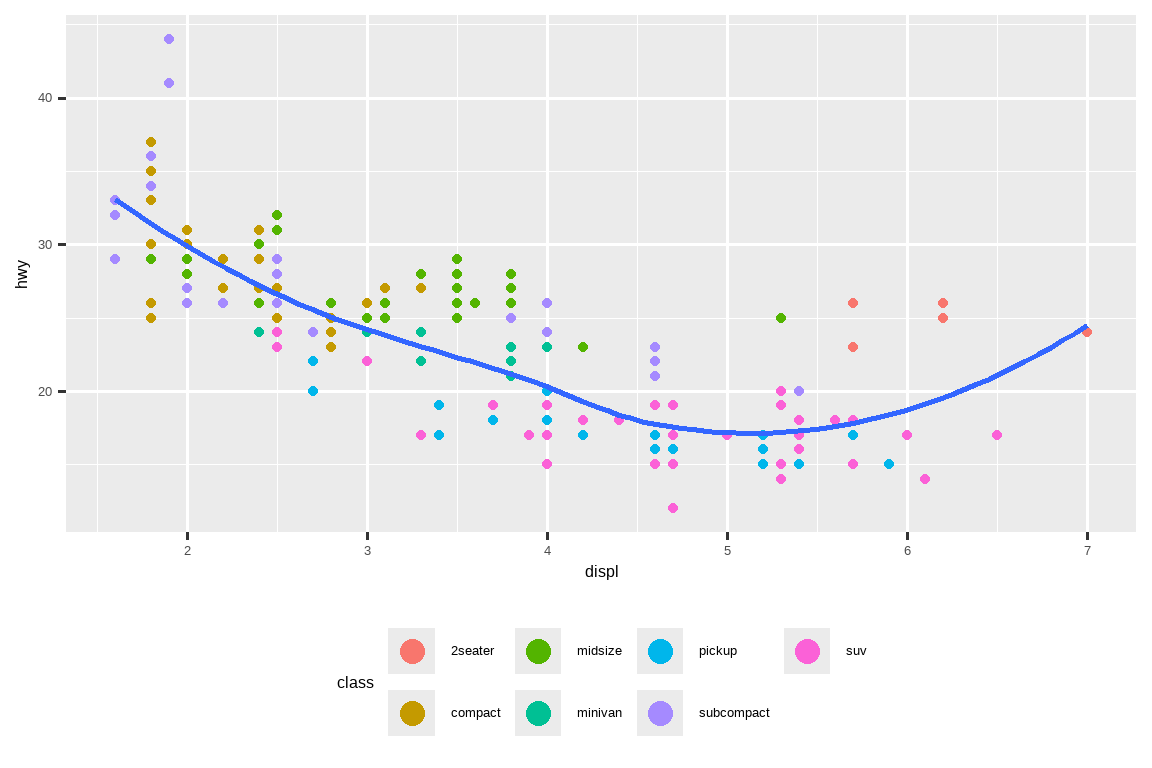

Scatterplot of highway fuel efficiency versus engine size of cars where points are colored based on class of car. Overlaid on the plot is a smooth curve. The legend is in the bottom and classes are listed horizontally in two rows. The points in the legend are larger than the points in the plot.

Note that the name of the argument in guides() matches the name of the aesthetic, just like in labs().
注意，guides() 中的参数名称与美学属性的名称相匹配，就像在 labs() 中一样。

11.4.4 Replacing a scale

Instead of just tweaking the details a little, you can instead replace the scale altogether. There are two types of scales you’re mostly likely to want to switch out: continuous position scales and color scales. Fortunately, the same principles apply to all the other aesthetics, so once you’ve mastered position and color, you’ll be able to quickly pick up other scale replacements.
你不仅可以微调细节，还可以完全替换整个标度。你最可能想要更换的两种标度是：连续位置标度和颜色标度。幸运的是，同样的原则也适用于所有其他美学属性，所以一旦你掌握了位置和颜色，你就能很快学会其他标度的替换。

It’s very useful to plot transformations of your variable. For example, it’s easier to see the precise relationship between carat and price if we log transform them:
对你的变量进行变换后绘图非常有用。例如，如果我们对 carat 和 price 进行对数变换，就更容易看清它们之间的精确关系：

# Left
ggplot(diamonds, aes(x = carat, y = price)) +
  geom_bin2d()

# Right
ggplot(diamonds, aes(x = log10(carat), y = log10(price))) +
  geom_bin2d()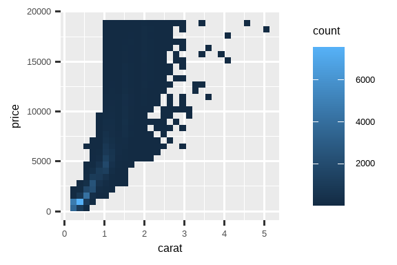

Two plots of price versus carat of diamonds. Data binned and the color of the rectangles representing each bin based on the number of points that fall into that bin. In the plot on the right, price and carat values are logged and the axis labels shows the logged values.

However, the disadvantage of this transformation is that the axes are now labelled with the transformed values, making it hard to interpret the plot. Instead of doing the transformation in the aesthetic mapping, we can instead do it with the scale. This is visually identical, except the axes are labelled on the original data scale.
然而，这种变换的缺点是坐标轴现在用变换后的值来标记，这使得图表难以解读。我们可以在标度中进行变换，而不是在美学映射中进行。这样在视觉上是相同的，但坐标轴会以原始数据标度进行标记。

ggplot(diamonds, aes(x = carat, y = price)) +
  geom_bin2d() + 
  scale_x_log10() + 
  scale_y_log10()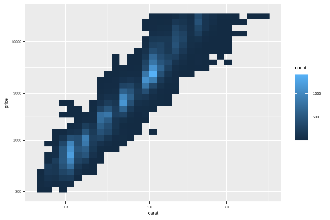

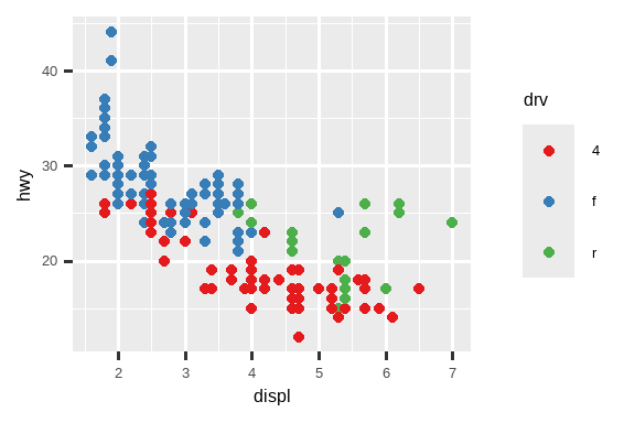
Plot of price versus carat of diamonds. Data binned and the color of the rectangles representing each bin based on the number of points that fall into that bin. The axis labels are on the original data scale.

Another scale that is frequently customized is color. The default categorical scale picks colors that are evenly spaced around the color wheel. Useful alternatives are the ColorBrewer scales which have been hand tuned to work better for people with common types of color blindness. The two plots below look similar, but there is enough difference in the shades of red and green that the dots on the right can be distinguished even by people with red-green color blindness.¹
另一个经常被定制的标度是颜色。默认的分类标度会选择在色轮上均匀分布的颜色。一些有用的替代方案是 ColorBrewer 标度，这些标度经过手工调整，对患有常见色盲类型的人更加友好。下面的两幅图看起来相似，但红色和绿色的色度有足够的差异，即使是红绿色盲的人也能区分右图中的点。¹

ggplot(mpg, aes(x = displ, y = hwy)) +
  geom_point(aes(color = drv))

ggplot(mpg, aes(x = displ, y = hwy)) +
  geom_point(aes(color = drv)) +
  scale_color_brewer(palette = "Set1")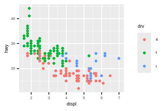

Two scatterplots of highway mileage versus engine size where points are colored by drive type. The plot on the left uses the default ggplot2 color palette and the plot on the right uses a different color palette.

Don’t forget simpler techniques for improving accessibility. If there are just a few colors, you can add a redundant shape mapping. This will also help ensure your plot is interpretable in black and white.
不要忘记使用更简单的技术来提高可访问性。如果只有几种颜色，你可以添加一个冗余的形状映射。这也有助于确保你的图在黑白模式下也是可以理解的。

ggplot(mpg, aes(x = displ, y = hwy)) +
  geom_point(aes(color = drv, shape = drv)) +
  scale_color_brewer(palette = "Set1")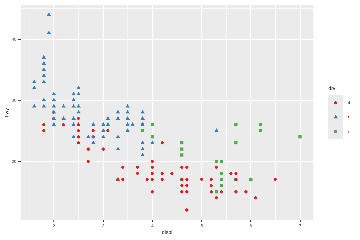

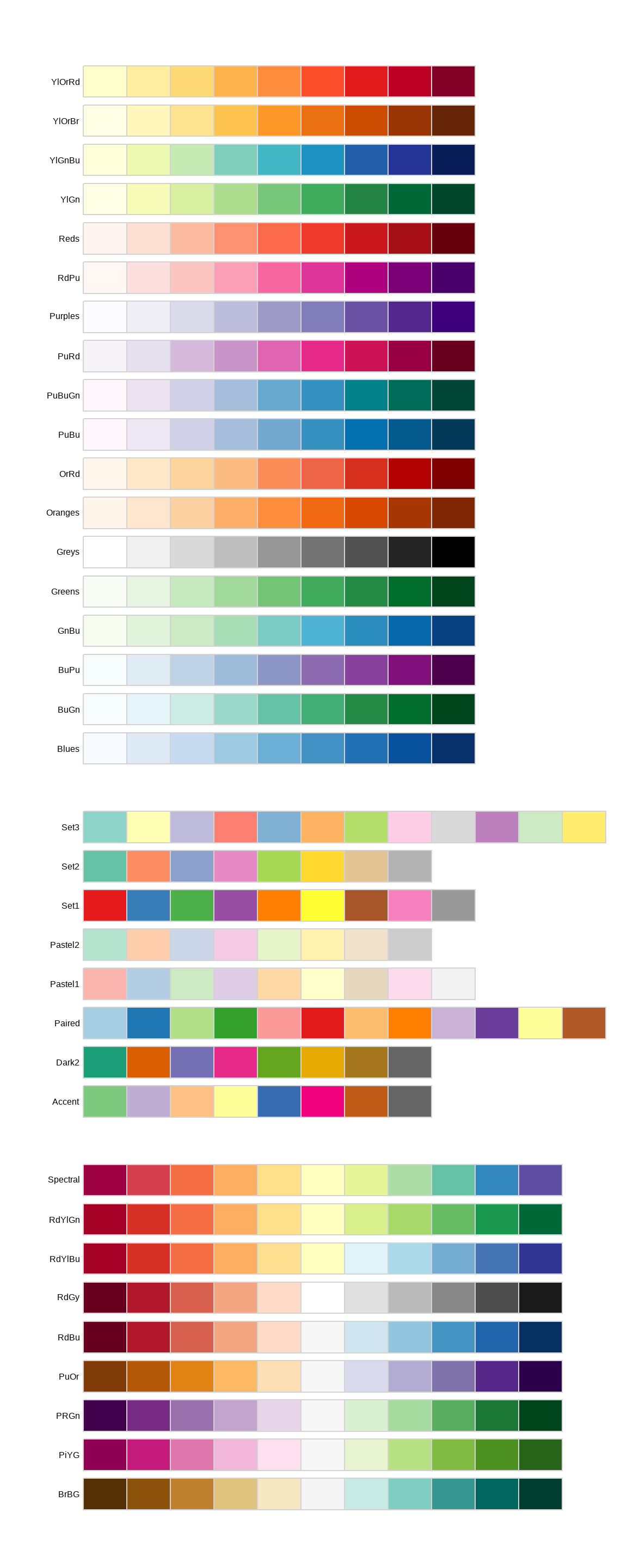
Scatterplot of highway mileage versus engine size where both color and shape of points are based on drive type. The color palette is not the default ggplot2 palette.

The ColorBrewer scales are documented online at https://colorbrewer2.org/ and made available in R via the RColorBrewer package, by Erich Neuwirth. Figure 11.1 shows the complete list of all palettes. The sequential (top) and diverging (bottom) palettes are particularly useful if your categorical values are ordered, or have a “middle”. This often arises if you’ve used cut() to make a continuous variable into a categorical variable.
ColorBrewer 色阶的文档可以在线查看：https://colorbrewer2.org/，并通过 Erich Neuwirth 开发的 RColorBrewer 包在 R 中使用。Figure 11.1 展示了所有调色板的完整列表。如果你的分类值是有序的，或者有一个“中间值”，那么顺序（顶部）和发散（底部）调色板就特别有用。这种情况通常发生在你使用 cut() 函数将连续变量转换为分类变量时。

All colorBrewer scales. One group goes from light to dark colors. Another group is a set of non ordinal colors. And the last group has diverging scales (from dark to light to dark again). Within each set there are a number of palettes. — Figure 11.1: All colorBrewer scales.

When you have a predefined mapping between values and colors, use scale_color_manual(). For example, if we map presidential party to color, we want to use the standard mapping of red for Republicans and blue for Democrats. One approach for assigning these colors is using hex color codes:
当你有一个预定义的值与颜色之间的映射时，请使用 scale_color_manual()。例如，如果我们将总统的党派映射到颜色，我们希望使用标准的映射：共和党为红色，民主党为蓝色。分配这些颜色的一种方法是使用十六进制颜色代码：

presidential |>
  mutate(id = 33 + row_number()) |>
  ggplot(aes(x = start, y = id, color = party)) +
  geom_point() +
  geom_segment(aes(xend = end, yend = id)) +
  scale_color_manual(values = c(Republican = "#E81B23", Democratic = "#00AEF3"))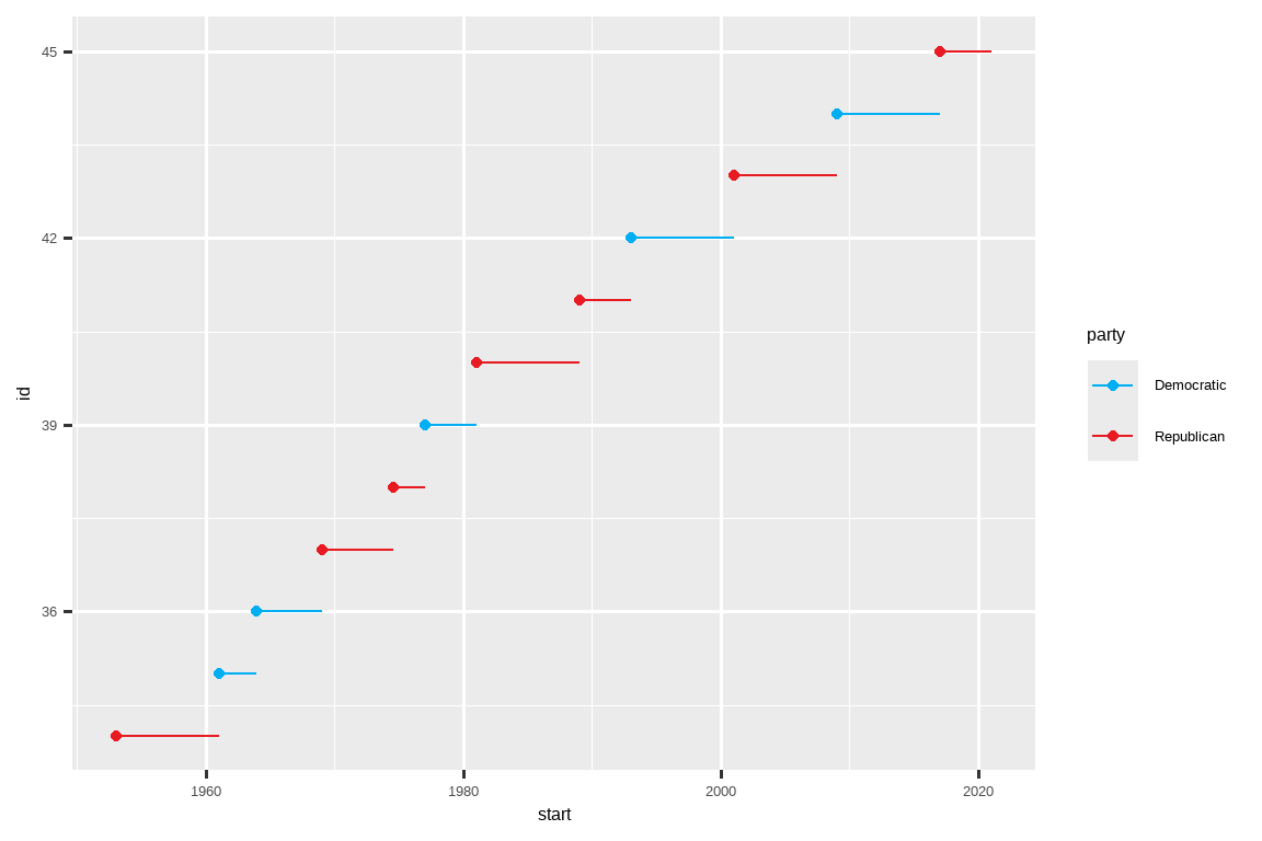

For continuous color, you can use the built-in scale_color_gradient() or scale_fill_gradient(). If you have a diverging scale, you can use scale_color_gradient2(). That allows you to give, for example, positive and negative values different colors. That’s sometimes also useful if you want to distinguish points above or below the mean.
对于连续颜色，你可以使用内置的 scale_color_gradient() 或 scale_fill_gradient()。如果你有一个发散型标度，你可以使用 scale_color_gradient2()。这允许你，例如，给正值和负值赋予不同的颜色。如果你想区分平均值以上或以下的点，这有时也很有用。

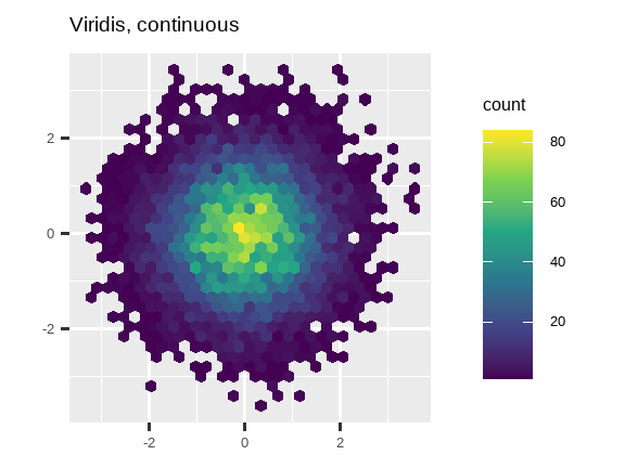
Another option is to use the viridis color scales. The designers, Nathaniel Smith and Stéfan van der Walt, carefully tailored continuous color schemes that are perceptible to people with various forms of color blindness as well as perceptually uniform in both color and black and white. These scales are available as continuous (c), discrete (d), and binned (b) palettes in ggplot2.
另一个选择是使用 viridis 颜色标度。其设计者 Nathaniel Smith 和 Stéfan van der Walt 精心设计了连续的颜色方案，这些方案对于各种形式的色盲人士来说都是可感知的，并且在彩色和黑白模式下都具有感知上的均匀性。这些标度在 ggplot2 中以连续 (c)、离散 (d) 和分箱 (b) 调色板的形式提供。

df <- tibble(
  x = rnorm(10000),
  y = rnorm(10000)
)

ggplot(df, aes(x, y)) +
  geom_hex() +
  coord_fixed() +
  labs(title = "Default, continuous", x = NULL, y = NULL)

ggplot(df, aes(x, y)) +
  geom_hex() +
  coord_fixed() +
  scale_fill_viridis_c() +
  labs(title = "Viridis, continuous", x = NULL, y = NULL)

ggplot(df, aes(x, y)) +
  geom_hex() +
  coord_fixed() +
  scale_fill_viridis_b() +
  labs(title = "Viridis, binned", x = NULL, y = NULL)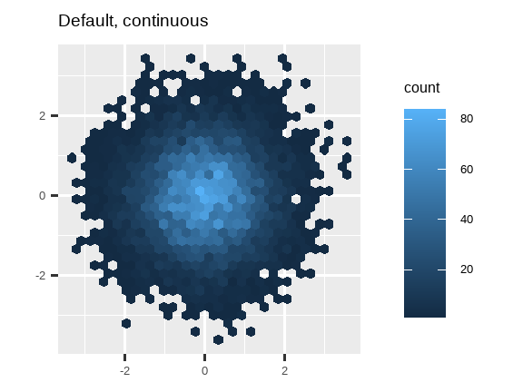

Three hex plots where the color of the hexes show the number of observations that fall into that hex bin. The first plot uses the default, continuous ggplot2 scale. The second plot uses the viridis, continuous scale, and the third plot uses the viridis, binned scale.

Note that all color scales come in two varieties: scale_color_*() and scale_fill_*() for the color and fill aesthetics respectively (the color scales are available in both UK and US spellings).
请注意，所有颜色标度都有两种变体：scale_color_*() 和 scale_fill_*()，分别对应 color 和 fill 美学属性（颜色标度提供英式和美式两种拼写）。

11.4.5 Zooming

There are three ways to control the plot limits:
有三种方法可以控制图的界限：

Adjusting what data are plotted.
调整被绘制的数据。
Setting the limits in each scale.
在每个标度中设置范围（limits）。
Setting xlim and ylim in coord_cartesian().
在 coord_cartesian() 中设置 xlim 和 ylim。

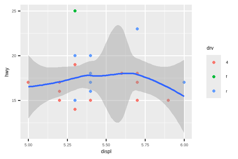
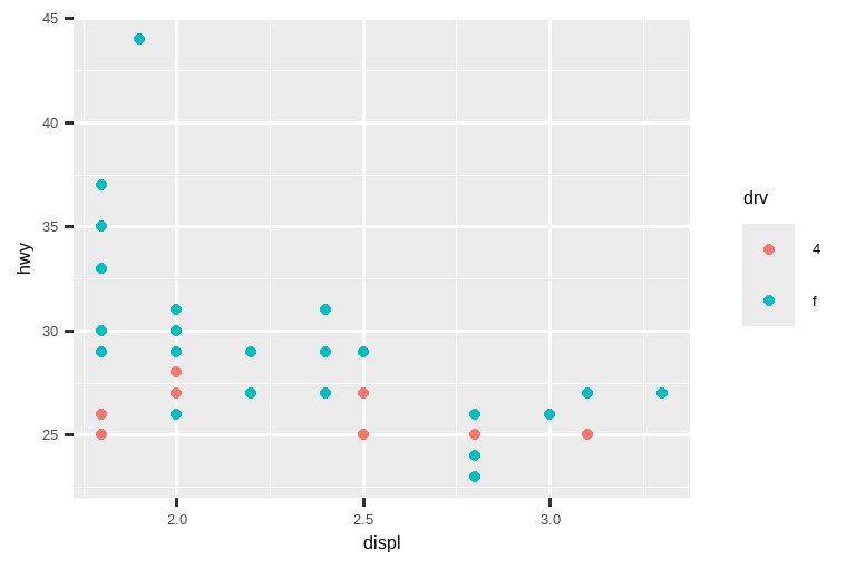
We’ll demonstrate these options in a series of plots. The plot on the left shows the relationship between engine size and fuel efficiency, colored by type of drive train. The plot on the right shows the same variables, but subsets the data that are plotted. Subsetting the data has affected the x and y scales as well as the smooth curve.
我们将通过一系列图表来演示这些选项。左边的图表显示了发动机尺寸和燃油效率之间的关系，并按驱动类型着色。右边的图表显示了相同的变量，但对绘制的数据进行了子集化。对数据进行子集化影响了 x 和 y 轴的标度以及平滑曲线。

# Left
ggplot(mpg, aes(x = displ, y = hwy)) +
  geom_point(aes(color = drv)) +
  geom_smooth()

# Right
mpg |>
  filter(displ >= 5 & displ <= 6 & hwy >= 10 & hwy <= 25) |>
  ggplot(aes(x = displ, y = hwy)) +
  geom_point(aes(color = drv)) +
  geom_smooth()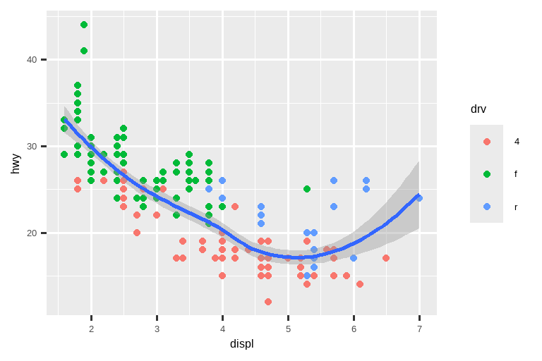

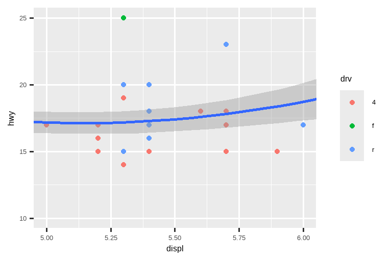
Let’s compare these to the two plots below where the plot on the left sets the limits on individual scales and the plot on the right sets them in coord_cartesian(). We can see that reducing the limits is equivalent to subsetting the data. Therefore, to zoom in on a region of the plot, it’s generally best to use coord_cartesian().
让我们将这些与下面的两张图进行比较，其中左边的图在单个标度上设置了 limits，而右边的图在 coord_cartesian() 中设置了它们。我们可以看到，缩小限制等同于对数据进行子集化。因此，要放大图的某个区域，通常最好使用 coord_cartesian()。

# Left
ggplot(mpg, aes(x = displ, y = hwy)) +
  geom_point(aes(color = drv)) +
  geom_smooth() +
  scale_x_continuous(limits = c(5, 6)) +
  scale_y_continuous(limits = c(10, 25))

# Right
ggplot(mpg, aes(x = displ, y = hwy)) +
  geom_point(aes(color = drv)) +
  geom_smooth() +
  coord_cartesian(xlim = c(5, 6), ylim = c(10, 25))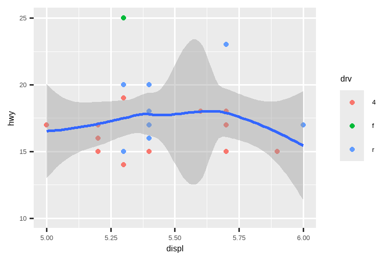

On the left, scatterplot of highway mileage vs. displacement, with displacement ranging from 5 to 6 and highway mileage ranging from 10 to 25. The smooth curve overlaid shows a trend that's slightly increasing first and then decreasing. On the right, same variables are plotted with the same limits, however the smooth curve overlaid shows a relatively flat trend with a slight increase at the end.

On the other hand, setting the limits on individual scales is generally more useful if you want to expand the limits, e.g., to match scales across different plots. For example, if we extract two classes of cars and plot them separately, it’s difficult to compare the plots because all three scales (the x-axis, the y-axis, and the color aesthetic) have different ranges.
另一方面，如果你想扩大范围，例如，为了在不同图之间匹配标度，那么在单个标度上设置 limits 通常更有用。例如，如果我们提取两类汽车并分别绘制它们，那么比较这些图会很困难，因为所有三个标度（x轴、y轴和颜色美学）都有不同的范围。

suv <- mpg |> filter(class == "suv")
compact <- mpg |> filter(class == "compact")

# Left
ggplot(suv, aes(x = displ, y = hwy, color = drv)) +
  geom_point()

# Right
ggplot(compact, aes(x = displ, y = hwy, color = drv)) +
  geom_point()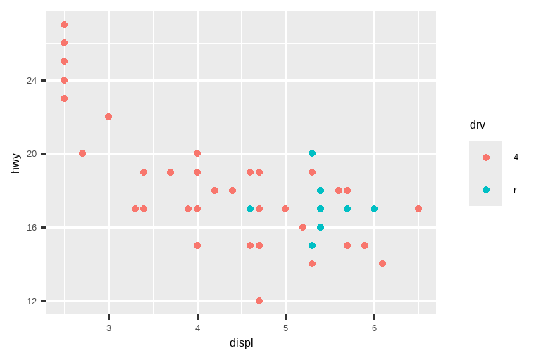

One way to overcome this problem is to share scales across multiple plots, training the scales with the limits of the full data.
克服这个问题的一种方法是在多个图之间共享标度，使用完整数据的 limits 来“训练”这些标度。

x_scale <- scale_x_continuous(limits = range(mpg$displ))
y_scale <- scale_y_continuous(limits = range(mpg$hwy))
col_scale <- scale_color_discrete(limits = unique(mpg$drv))

# Left
ggplot(suv, aes(x = displ, y = hwy, color = drv)) +
  geom_point() +
  x_scale +
  y_scale +
  col_scale

# Right
ggplot(compact, aes(x = displ, y = hwy, color = drv)) +
  geom_point() +
  x_scale +
  y_scale +
  col_scale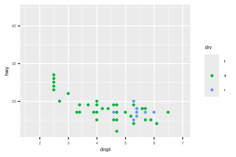

In this particular case, you could have simply used faceting, but this technique is useful more generally, if for instance, you want to spread plots over multiple pages of a report.
在这个特定的案例中，你本可以简单地使用分面，但这种技术在更普遍的情况下也很有用，例如，当你想将图表分布在报告的多个页面上时。

11.4.6 Exercises

Why doesn’t the following code override the default scale?

df <- tibble(
  x = rnorm(10000),
  y = rnorm(10000)
)

ggplot(df, aes(x, y)) +
  geom_hex() +
  scale_color_gradient(low = "white", high = "red") +
  coord_fixed()

What is the first argument to every scale? How does it compare to labs()?
Change the display of the presidential terms by:
1. Combining the two variants that customize colors and x axis breaks.
2. Improving the display of the y axis.
3. Labelling each term with the name of the president.
4. Adding informative plot labels.
5. Placing breaks every 4 years (this is trickier than it seems!).
First, create the following plot. Then, modify the code using override.aes to make the legend easier to see.
```
ggplot(diamonds, aes(x = carat, y = price)) +
  geom_point(aes(color = cut), alpha = 1/20)
```

11.5 Themes

Finally, you can customize the non-data elements of your plot with a theme:
最后，你可以使用主题 (theme) 来自定义图形中的非数据元素：

ggplot(mpg, aes(x = displ, y = hwy)) +
  geom_point(aes(color = class)) +
  geom_smooth(se = FALSE) +
  theme_bw()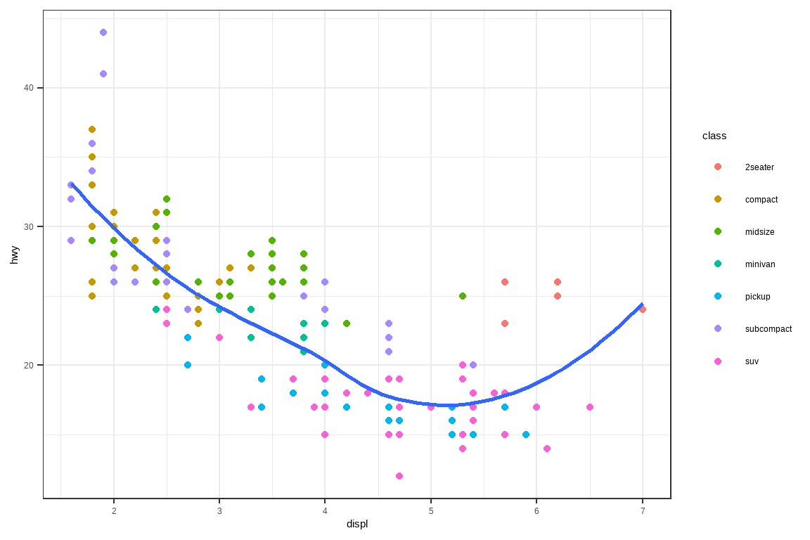

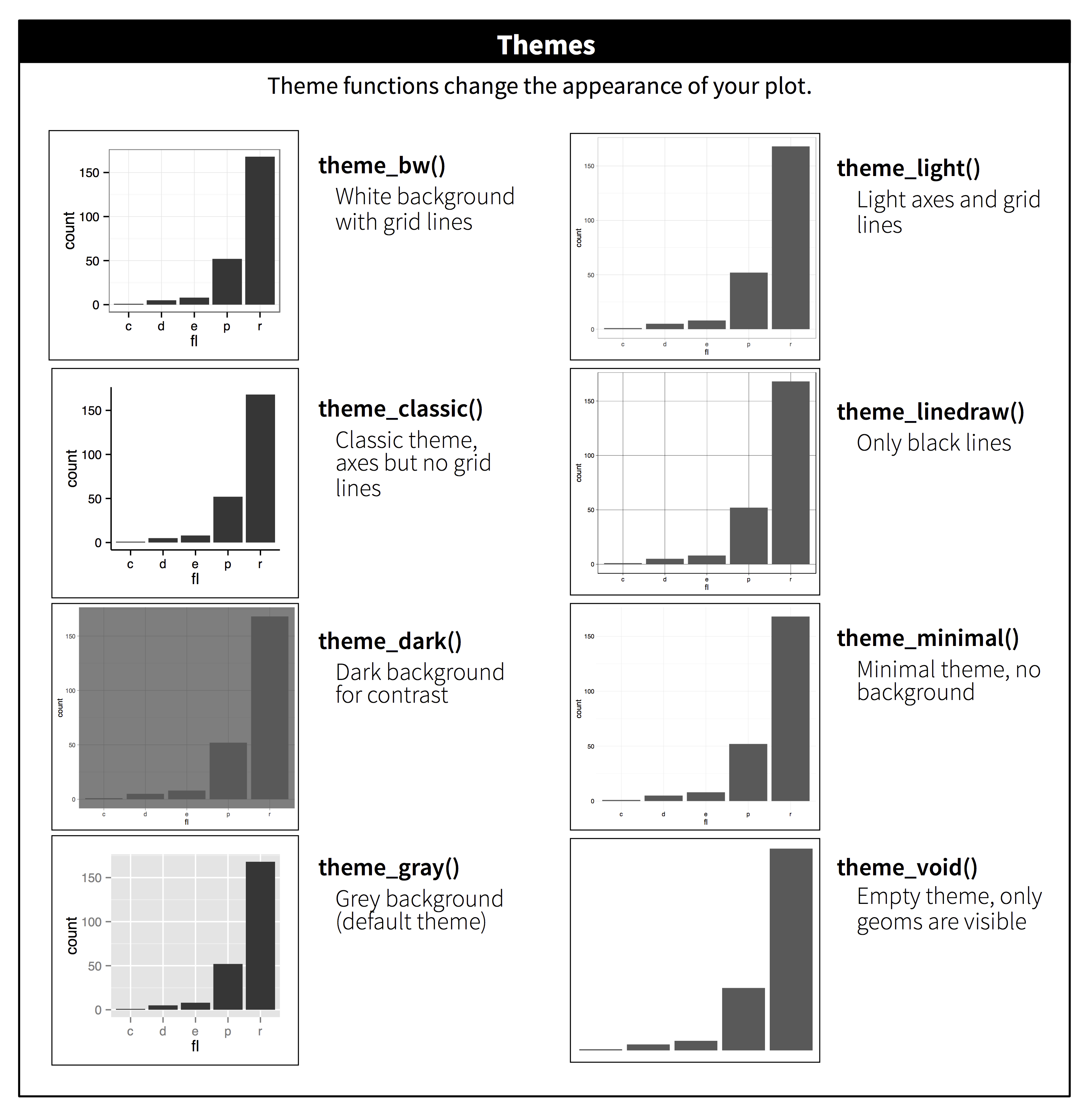
Scatterplot of highway mileage vs. displacement of cars, colored by class of car. The plot background is white, with gray grid lines.

ggplot2 includes the eight themes shown in Figure 11.2, with theme_gray() as the default.² Many more are included in add-on packages like ggthemes (https://jrnold.github.io/ggthemes), by Jeffrey Arnold. You can also create your own themes, if you are trying to match a particular corporate or journal style.
ggplot2 包含了 Figure 11.2 中显示的八个主题，其中 theme_gray() 是默认主题。² 还有更多主题包含在附加包中，例如 Jeffrey Arnold 开发的 ggthemes (https://jrnold.github.io/ggthemes)。如果你想匹配特定的公司或期刊风格，也可以创建自己的主题。

Eight barplots created with ggplot2, each with one of the eight built-in themes: theme_bw() - White background with grid lines, theme_light() - Light axes and grid lines, theme_classic() - Classic theme, axes but no grid lines, theme_linedraw() - Only black lines, theme_dark() - Dark background for contrast, theme_minimal() - Minimal theme, no background, theme_gray() - Gray background (default theme), theme_void() - Empty theme, only geoms are visible. — Figure 11.2: The eight themes built-in to ggplot2.

It’s also possible to control individual components of each theme, like the size and color of the font used for the y axis. We’ve already seen that legend.position controls where the legend is drawn. There are many other aspects of the legend that can be customized with theme(). For example, in the plot below we change the direction of the legend as well as put a black border around it. Note that customization of the legend box and plot title elements of the theme are done with element_*() functions. These functions specify the styling of non-data components, e.g., the title text is bolded in the face argument of element_text() and the legend border color is defined in the color argument of element_rect(). The theme elements that control the position of the title and the caption are plot.title.position and plot.caption.position, respectively. In the following plot these are set to "plot" to indicate these elements are aligned to the entire plot area, instead of the plot panel (the default). A few other helpful theme() components are used to change the placement for format of the title and caption text.
也可以控制每个主题的单个组件，比如 y 轴使用的字体大小和颜色。我们已经看到 legend.position 控制图例的绘制位置。图例的许多其他方面也可以用 theme() 来定制。例如，在下面的图中，我们改变了图例的方向，并给它加上了黑色的边框。注意，图例框和图标题等主题元素的定制是通过 element_*() 函数完成的。这些函数指定了非数据组件的样式，例如，标题文本在 element_text() 的 face 参数中被加粗，图例边框颜色在 element_rect() 的 color 参数中被定义。控制标题和说明文字位置的主题元素分别是 plot.title.position 和 plot.caption.position。在下面的图中，这些被设置为 "plot"，表示这些元素与整个绘图区域对齐，而不是绘图面板（默认值）。还使用了一些其他有用的 theme() 组件来更改标题和说明文字的位置格式。

ggplot(mpg, aes(x = displ, y = hwy, color = drv)) +
  geom_point() +
  labs(
    title = "Larger engine sizes tend to have lower fuel economy",
    caption = "Source: https://fueleconomy.gov."
  ) +
  theme(
    legend.position = c(0.6, 0.7),
    legend.direction = "horizontal",
    legend.box.background = element_rect(color = "black"),
    plot.title = element_text(face = "bold"),
    plot.title.position = "plot",
    plot.caption.position = "plot",
    plot.caption = element_text(hjust = 0)
  )
#> Warning: A numeric `legend.position` argument in `theme()` was deprecated in ggplot2
#> 3.5.0.
#> ℹ Please use the `legend.position.inside` argument of `theme()` instead.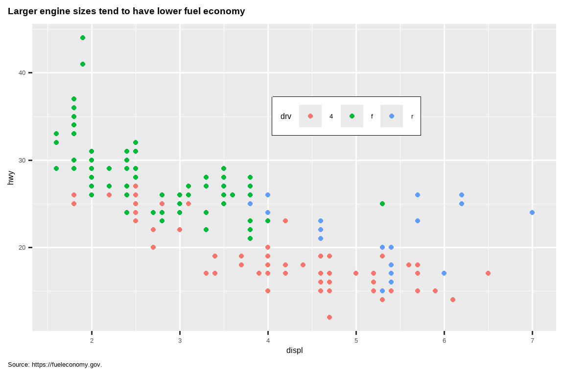

Scatterplot of highway fuel efficiency versus engine size of cars, colored by drive. The plot is titled 'Larger engine sizes tend to have lower fuel economy' with the caption pointing to the source of the data, fueleconomy.gov. The caption and title are left justified, the legend is inside of the plot with a black border.

For an overview of all theme() components, see help with ?theme. The ggplot2 book is also a great place to go for the full details on theming.
要了解所有 theme() 组件的概览，请查看 ?theme 的帮助文档。ggplot2 book 也是一个了解主题设置全部细节的好去处。

11.5.1 Exercises

Pick a theme offered by the ggthemes package and apply it to the last plot you made.
Make the axis labels of your plot blue and bolded.

11.6 Layout

So far we talked about how to create and modify a single plot. What if you have multiple plots you want to lay out in a certain way? The patchwork package allows you to combine separate plots into the same graphic. We loaded this package earlier in the chapter.
到目前为止，我们讨论了如何创建和修改单个图。但如果你有多个图，并希望以某种特定方式布局它们，该怎么办呢？patchwork 包允许你将多个独立的图组合成一个图形。我们在本章前面已经加载了这个包。

To place two plots next to each other, you can simply add them to each other. Note that you first need to create the plots and save them as objects (in the following example they’re called p1 and p2). Then, you place them next to each other with +.
要将两个图并排放置，你只需将它们相加即可。请注意，你首先需要创建这些图并将它们保存为对象（在下面的示例中，它们被称为 p1 和 p2）。然后，你用 + 将它们并排放置。

p1 <- ggplot(mpg, aes(x = displ, y = hwy)) + 
  geom_point() + 
  labs(title = "Plot 1")
p2 <- ggplot(mpg, aes(x = drv, y = hwy)) + 
  geom_boxplot() + 
  labs(title = "Plot 2")
p1 + p2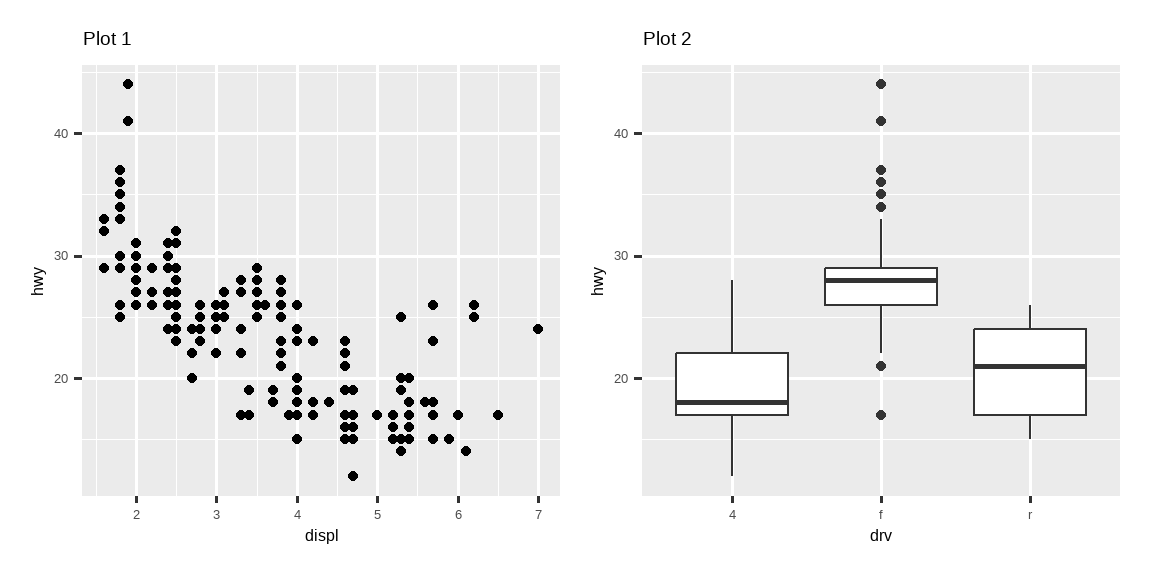

Two plots (a scatterplot of highway mileage versus engine size and a side-by-side boxplots of highway mileage versus drive train) placed next to each other.

It’s important to note that in the above code chunk we did not use a new function from the patchwork package. Instead, the package added a new functionality to the + operator.
需要注意的是，在上面的代码块中，我们并未使用 patchwork 包中的新函数。相反，该包为 + 运算符添加了新的功能。

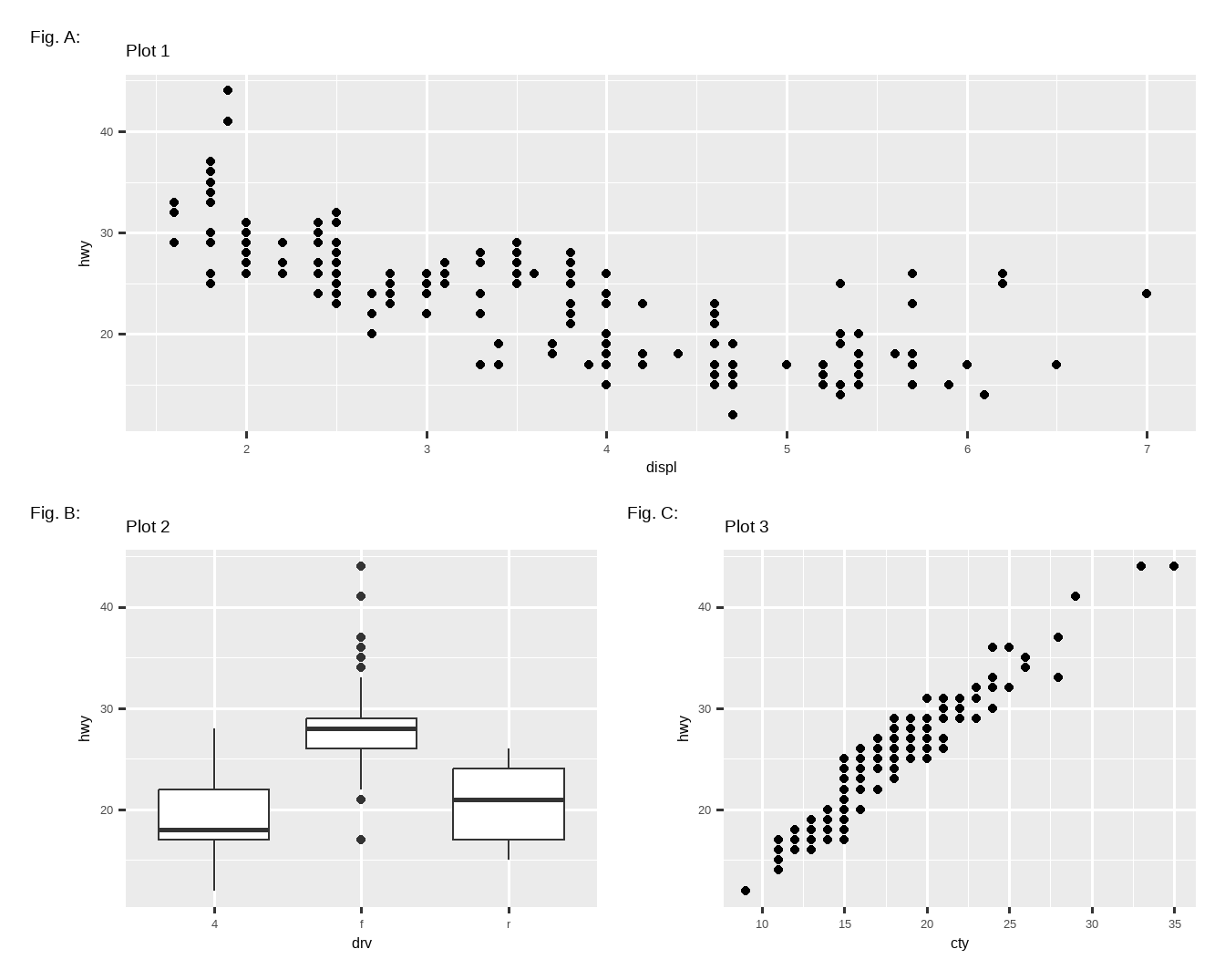
You can also create complex plot layouts with patchwork. In the following, | places the p1 and p3 next to each other and / moves p2 to the next line.
你还可以使用 patchwork 创建复杂的图形布局。在下文中，| 将 p1 和 p3 并排放置，而 / 将 p2 移到下一行。

p3 <- ggplot(mpg, aes(x = cty, y = hwy)) + 
  geom_point() + 
  labs(title = "Plot 3")
(p1 | p3) / p2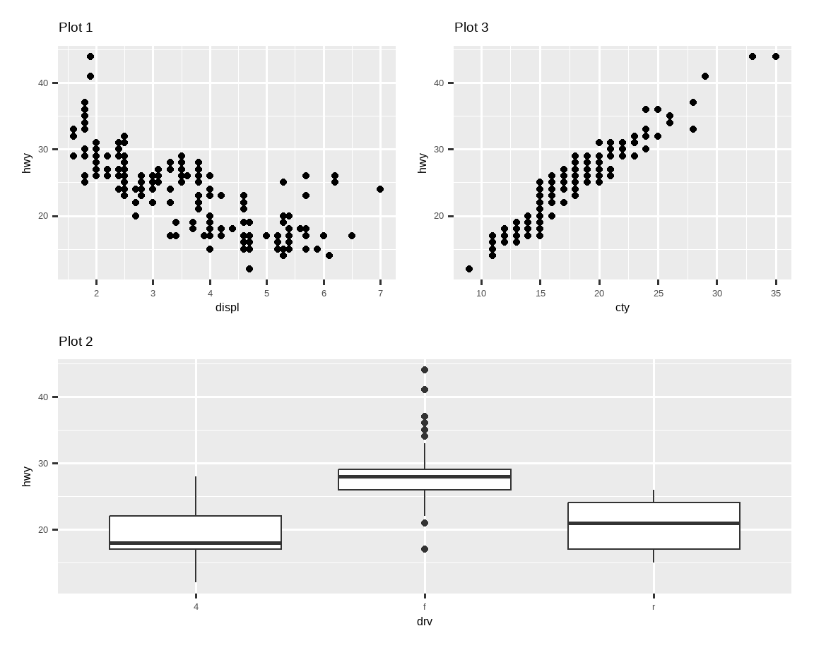

Three plots laid out such that first and third plot are next to each other and the second plot stretched beneath them. The first plot is a scatterplot of highway mileage versus engine size, the third plot is a scatterplot of highway mileage versus city mileage, and the second plot is side-by-side boxplots of highway mileage versus drive train).

Additionally, patchwork allows you to collect legends from multiple plots into one common legend, customize the placement of the legend as well as dimensions of the plots, and add a common title, subtitle, caption, etc. to your plots. Below we create 5 plots. We have turned off the legends on the box plots and the scatterplot and collected the legends for the density plots at the top of the plot with & theme(legend.position = "top"). Note the use of the & operator here instead of the usual +. This is because we’re modifying the theme for the patchwork plot as opposed to the individual ggplots. The legend is placed on top, inside the guide_area(). Finally, we have also customized the heights of the various components of our patchwork – the guide has a height of 1, the box plots 3, density plots 2, and the faceted scatterplot 4. Patchwork divides up the area you have allotted for your plot using this scale and places the components accordingly.
此外，patchwork 允许你将多个图的图例收集到一个公共图例中，自定义图例的位置以及图的尺寸，并为你的图添加公共的标题、副标题、说明等。下面我们创建 5 个图。我们关闭了箱线图和散点图的图例，并使用 & theme(legend.position = "top") 将密度图的图例收集到图的顶部。注意这里使用了 & 操作符而不是通常的 +。这是因为我们正在修改 patchwork 图的主题，而不是单个 ggplot。图例被放置在顶部，在 guide_area() 内部。最后，我们还自定义了 patchwork 各个组件的高度——引导区高度为 1，箱线图为 3，密度图为 2，分面散点图为 4。Patchwork 使用这个比例来划分你为图分配的区域，并相应地放置组件。

p1 <- ggplot(mpg, aes(x = drv, y = cty, color = drv)) + 
  geom_boxplot(show.legend = FALSE) + 
  labs(title = "Plot 1")

p2 <- ggplot(mpg, aes(x = drv, y = hwy, color = drv)) + 
  geom_boxplot(show.legend = FALSE) + 
  labs(title = "Plot 2")

p3 <- ggplot(mpg, aes(x = cty, color = drv, fill = drv)) + 
  geom_density(alpha = 0.5) + 
  labs(title = "Plot 3")

p4 <- ggplot(mpg, aes(x = hwy, color = drv, fill = drv)) + 
  geom_density(alpha = 0.5) + 
  labs(title = "Plot 4")

p5 <- ggplot(mpg, aes(x = cty, y = hwy, color = drv)) + 
  geom_point(show.legend = FALSE) + 
  facet_wrap(~drv) +
  labs(title = "Plot 5")

(guide_area() / (p1 + p2) / (p3 + p4) / p5) +
  plot_annotation(
    title = "City and highway mileage for cars with different drive trains",
    caption = "Source: https://fueleconomy.gov."
  ) +
  plot_layout(
    guides = "collect",
    heights = c(1, 3, 2, 4)
    ) &
  theme(legend.position = "top")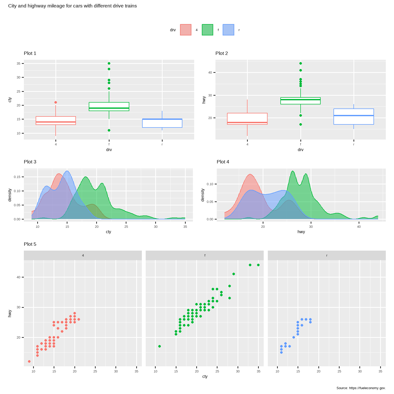

Five plots laid out such that first two plots are next to each other. Plots three and four are underneath them. And the fifth plot stretches under them. The patchworked plot is titled "City and highway mileage for cars with different drive trains" and captioned "Source: https://fueleconomy.gov". The first two plots are side-by-side box plots. Plots 3 and 4 are density plots. And the fifth plot is a faceted scatterplot. Each of these plots show geoms colored by drive train, but the patchworked plot has only one legend that applies to all of them, above the plots and beneath the title.

If you’d like to learn more about combining and layout out multiple plots with patchwork, we recommend looking through the guides on the package website: https://patchwork.data-imaginist.com.
如果你想了解更多关于使用 patchwork 组合和布局多个图的信息，我们建议你浏览该包网站上的指南：https://patchwork.data-imaginist.com。

11.6.1 Exercises

What happens if you omit the parentheses in the following plot layout. Can you explain why this happens?

p1 <- ggplot(mpg, aes(x = displ, y = hwy)) + 
  geom_point() + 
  labs(title = "Plot 1")
p2 <- ggplot(mpg, aes(x = drv, y = hwy)) + 
  geom_boxplot() + 
  labs(title = "Plot 2")
p3 <- ggplot(mpg, aes(x = cty, y = hwy)) + 
  geom_point() + 
  labs(title = "Plot 3")

(p1 | p2) / p3

Using the three plots from the previous exercise, recreate the following patchwork.

11.7 Summary

In this chapter you’ve learned about adding plot labels such as title, subtitle, caption as well as modifying default axis labels, using annotation to add informational text to your plot or to highlight specific data points, customizing the axis scales, and changing the theme of your plot. You’ve also learned about combining multiple plots in a single graph using both simple and complex plot layouts.
在本章中，你学习了添加图形标签（如标题、副标题、说明文字）以及修改默认坐标轴标签、使用注释为图形添加信息性文本或突出显示特定数据点、自定义坐标轴标度和更改图形主题。你还学习了使用简单和复杂的图形布局将多个图形组合成一个图形。

While you’ve so far learned about how to make many different types of plots and how to customize them using a variety of techniques, we’ve barely scratched the surface of what you can create with ggplot2. If you want to get a comprehensive understanding of ggplot2, we recommend reading the book, ggplot2: Elegant Graphics for Data Analysis. Other useful resources are the R Graphics Cookbook by Winston Chang and Fundamentals of Data Visualization by Claus Wilke.
到目前为止，你已经学会了如何制作多种不同类型的图，以及如何使用各种技术对其进行自定义，但我们对 ggplot2 能创建的内容还只是浅尝辄止。如果你想全面了解 ggplot2，我们推荐阅读 ggplot2: Elegant Graphics for Data Analysis 这本书。其他有用的资源包括 Winston Chang 的 R Graphics Cookbook 和 Claus Wilke 的 Fundamentals of Data Visualization。

You can use a tool like SimDaltonism to simulate color blindness to test these images.↩︎
Many people wonder why the default theme has a gray background. This was a deliberate choice because it puts the data forward while still making the grid lines visible. The white grid lines are visible (which is important because they significantly aid position judgments), but they have little visual impact and we can easily tune them out. The gray background gives the plot a similar typographic color to the text, ensuring that the graphics fit in with the flow of a document without jumping out with a bright white background. Finally, the gray background creates a continuous field of color which ensures that the plot is perceived as a single visual entity.↩︎