5  Data tidying

5.1 Introduction

“Happy families are all alike; every unhappy family is unhappy in its own way.”
— Leo Tolstoy
“幸福的家庭都是相似的；不幸的家庭各有各的不幸。”
— 列夫·托尔斯泰

“Tidy datasets are all alike, but every messy dataset is messy in its own way.”
— Hadley Wickham
“整洁的数据集都是相似的，但每个凌乱的数据集各有各的凌乱之处。”
— Hadley Wickham

In this chapter, you will learn a consistent way to organize your data in R using a system called tidy data. Getting your data into this format requires some work up front, but that work pays off in the long term. Once you have tidy data and the tidy tools provided by packages in the tidyverse, you will spend much less time munging data from one representation to another, allowing you to spend more time on the data questions you care about.
在本章中，你将学习一种在 R 中组织数据的一致性方法，这个系统被称为整洁数据 (tidy data)。 将数据整理成这种格式需要一些前期工作，但从长远来看，这些工作是值得的。 一旦你拥有了整洁的数据以及 tidyverse 中各个包提供的整洁工具，你将花费更少的时间在不同数据表示形式之间进行转换，从而可以投入更多时间来关注你所关心的数据问题。

In this chapter, you’ll first learn the definition of tidy data and see it applied to a simple toy dataset. Then we’ll dive into the primary tool you’ll use for tidying data: pivoting. Pivoting allows you to change the form of your data without changing any of the values.
在本章中，你将首先学习整洁数据的定义，并看到它如何应用于一个简单的示例数据集。 然后，我们将深入探讨用于整理数据的主要工具：透视 (pivoting)。 透视允许你在不改变任何值的情况下改变数据的形态。

5.1.1 Prerequisites

In this chapter, we’ll focus on tidyr, a package that provides a bunch of tools to help tidy up your messy datasets. tidyr is a member of the core tidyverse.
在本章中，我们将重点介绍 tidyr，这个包提供了一系列工具来帮助你整理凌乱的数据集。 tidyr 是核心 tidyverse 的成员之一。

library(tidyverse)

From this chapter on, we’ll suppress the loading message from library(tidyverse).
从本章开始，我们将抑制 library(tidyverse) 的加载消息。

5.2 Tidy data

You can represent the same underlying data in multiple ways. The example below shows the same data organized in three different ways. Each dataset shows the same values of four variables: country, year, population, and number of documented cases of TB (tuberculosis), but each dataset organizes the values in a different way.
你可以用多种方式表示相同的基础数据。 下面的示例展示了以三种不同方式组织的相同数据。 每个数据集都显示了四个变量的相同值：country (国家)、year (年份)、population (人口) 和记录在案的 cases (结核病病例数)，但每个数据集以不同的方式组织这些值。

table1
#> # A tibble: 6 × 4
#>   country      year  cases population
#>   <chr>       <dbl>  <dbl>      <dbl>
#> 1 Afghanistan  1999    745   19987071
#> 2 Afghanistan  2000   2666   20595360
#> 3 Brazil       1999  37737  172006362
#> 4 Brazil       2000  80488  174504898
#> 5 China        1999 212258 1272915272
#> 6 China        2000 213766 1280428583

table2
#> # A tibble: 12 × 4
#>   country      year type           count
#>   <chr>       <dbl> <chr>          <dbl>
#> 1 Afghanistan  1999 cases            745
#> 2 Afghanistan  1999 population  19987071
#> 3 Afghanistan  2000 cases           2666
#> 4 Afghanistan  2000 population  20595360
#> 5 Brazil       1999 cases          37737
#> 6 Brazil       1999 population 172006362
#> # ℹ 6 more rows

table3
#> # A tibble: 6 × 3
#>   country      year rate             
#>   <chr>       <dbl> <chr>            
#> 1 Afghanistan  1999 745/19987071     
#> 2 Afghanistan  2000 2666/20595360    
#> 3 Brazil       1999 37737/172006362  
#> 4 Brazil       2000 80488/174504898  
#> 5 China        1999 212258/1272915272
#> 6 China        2000 213766/1280428583

These are all representations of the same underlying data, but they are not equally easy to use. One of them, table1, will be much easier to work with inside the tidyverse because it’s tidy.
这些都是相同基础数据的不同表示形式，但它们的使用便利性并不相同。 其中之一，table1，在 tidyverse 中使用起来会容易得多，因为它是整洁的。

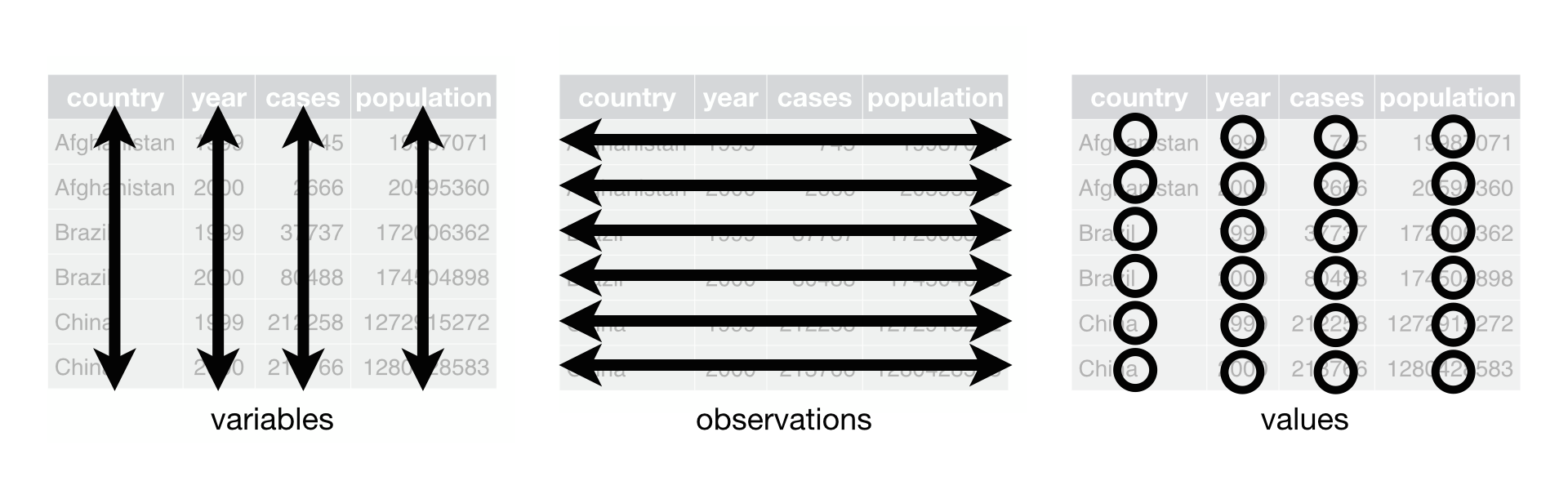
There are three interrelated rules that make a dataset tidy:
有三条相互关联的规则可以使数据集变得整洁：

1. Each variable is a column; each column is a variable.

2. Each observation is a row; each row is an observation.

3. Each value is a cell; each cell is a single value.

4. 每个变量是一列；每列是一个变量。

5. 每个观测是一行；每行是一个观测。

6. 每个值是一个单元格；每个单元格是一个值。

Figure 5.1 shows the rules visually.
Figure 5.1 直观地展示了这些规则。

Figure 5.1: The following three rules make a dataset tidy: variables are columns, observations are rows, and values are cells.

Why ensure that your data is tidy? There are two main advantages:
为什么要确保你的数据是整洁的？ 主要有两个优点：

1. There’s a general advantage to picking one consistent way of storing data. If you have a consistent data structure, it’s easier to learn the tools that work with it because they have an underlying uniformity.

2. There’s a specific advantage to placing variables in columns because it allows R’s vectorized nature to shine. As you learned in Section 3.3.1 and Section 3.5.2, most built-in R functions work with vectors of values. That makes transforming tidy data feel particularly natural.

3. 选择一种一致的数据存储方式具有普遍的优势。 如果你有一个一致的数据结构，学习与之配合的工具会更容易，因为它们具有内在的一致性。

4. 将变量放在列中有一个特定的优势，因为这能让 R 的向量化特性大放异彩。 正如你在 Section 3.3.1 和 Section 3.5.2 中学到的，大多数内置的 R 函数都处理值的向量。 这使得转换整洁的数据感觉特别自然。

dplyr, ggplot2, and all the other packages in the tidyverse are designed to work with tidy data. Here are a few small examples showing how you might work with table1.
dplyr、ggplot2 以及 tidyverse 中的所有其他包都是为处理整洁数据而设计的。 这里有几个小例子，展示了你如何使用 table1。

# Compute rate per 10,000
table1 |>
  mutate(rate = cases / population * 10000)
#> # A tibble: 6 × 5
#>   country      year  cases population  rate
#>   <chr>       <dbl>  <dbl>      <dbl> <dbl>
#> 1 Afghanistan  1999    745   19987071 0.373
#> 2 Afghanistan  2000   2666   20595360 1.29 
#> 3 Brazil       1999  37737  172006362 2.19 
#> 4 Brazil       2000  80488  174504898 4.61 
#> 5 China        1999 212258 1272915272 1.67 
#> 6 China        2000 213766 1280428583 1.67

# Compute total cases per year
table1 |> 
  group_by(year) |> 
  summarize(total_cases = sum(cases))
#> # A tibble: 2 × 2
#>    year total_cases
#>   <dbl>       <dbl>
#> 1  1999      250740
#> 2  2000      296920

# Visualize changes over time
ggplot(table1, aes(x = year, y = cases)) +
  geom_line(aes(group = country), color = "grey50") +
  geom_point(aes(color = country, shape = country)) +
  scale_x_continuous(breaks = c(1999, 2000)) # x-axis breaks at 1999 and 2000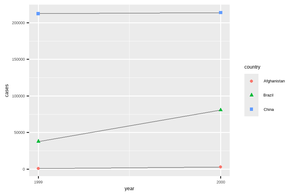

5.2.1 Exercises

1. For each of the sample tables, describe what each observation and each column represents.

2. Sketch out the process you’d use to calculate the rate for table2 and table3. You will need to perform four operations:

   1. Extract the number of TB cases per country per year.
   2. Extract the matching population per country per year.
   3. Divide cases by population, and multiply by 10000.
   4. Store back in the appropriate place.

   You haven’t yet learned all the functions you’d need to actually perform these operations, but you should still be able to think through the transformations you’d need.

5.3 Lengthening data

The principles of tidy data might seem so obvious that you wonder if you’ll ever encounter a dataset that isn’t tidy. Unfortunately, however, most real data is untidy. There are two main reasons:
整洁数据的原则可能看起来如此显而易见，以至于你可能会怀疑是否会遇到不整洁的数据集。 然而，不幸的是，大多数真实数据都是不整洁的。 主要有两个原因：

1. Data is often organized to facilitate some goal other than analysis. For example, it’s common for data to be structured to make data entry, not analysis, easy. 数据的组织方式通常是为了促进除分析之外的其他目标。 例如，为了方便数据录入而非分析而构建数据结构是很常见的。

2. Most people aren’t familiar with the principles of tidy data, and it’s hard to derive them yourself unless you spend a lot of time working with data.
   大多数人并不熟悉整洁数据的原则，除非你花大量时间处理数据，否则很难自己推导出这些原则。

This means that most real analyses will require at least a little tidying. You’ll begin by figuring out what the underlying variables and observations are. Sometimes this is easy; other times you’ll need to consult with the people who originally generated the data. Next, you’ll pivot your data into a tidy form, with variables in the columns and observations in the rows.
这意味着大多数实际分析至少需要一些整理工作。 你将首先弄清楚潜在的变量和观测值是什么。 有时这很简单；其他时候你可能需要咨询最初生成数据的人。 接下来，你将透视 (pivot) 你的数据，使其成为变量在列、观测在行的整洁形式。

tidyr provides two functions for pivoting data: pivot_longer() and pivot_wider(). We’ll first start with pivot_longer() because it’s the most common case. Let’s dive into some examples.
tidyr 提供了两个用于数据透视的函数：pivot_longer() 和 pivot_wider()。 我们将首先从 pivot_longer() 开始，因为这是最常见的情况。 让我们来看一些例子。

5.3.1 Data in column names

The billboard dataset records the billboard rank of songs in the year 2000:
billboard 数据集记录了 2000 年歌曲的 billboard 排行榜排名：

billboard
#> # A tibble: 317 × 79
#>   artist       track               date.entered   wk1   wk2   wk3   wk4   wk5
#>   <chr>        <chr>               <date>       <dbl> <dbl> <dbl> <dbl> <dbl>
#> 1 2 Pac        Baby Don't Cry (Ke… 2000-02-26      87    82    72    77    87
#> 2 2Ge+her      The Hardest Part O… 2000-09-02      91    87    92    NA    NA
#> 3 3 Doors Down Kryptonite          2000-04-08      81    70    68    67    66
#> 4 3 Doors Down Loser               2000-10-21      76    76    72    69    67
#> 5 504 Boyz     Wobble Wobble       2000-04-15      57    34    25    17    17
#> 6 98^0         Give Me Just One N… 2000-08-19      51    39    34    26    26
#> # ℹ 311 more rows
#> # ℹ 71 more variables: wk6 <dbl>, wk7 <dbl>, wk8 <dbl>, wk9 <dbl>, …

In this dataset, each observation is a song. The first three columns (artist, track and date.entered) are variables that describe the song. Then we have 76 columns (wk1-wk76) that describe the rank of the song in each week¹. Here, the column names are one variable (the week) and the cell values are another (the rank).
在这个数据集中，每个观测是一首歌曲。 前三列（artist、track 和 date.entered）是描述歌曲的变量。 然后我们有 76 列（wk1 到 wk76），描述了歌曲在每周的排名¹。 在这里，列名是一个变量（week），而单元格的值是另一个变量（rank）。

To tidy this data, we’ll use pivot_longer():
为了整理这个数据，我们将使用 pivot_longer()：

billboard |> 
  pivot_longer(
    cols = starts_with("wk"), 
    names_to = "week", 
    values_to = "rank"
  )
#> # A tibble: 24,092 × 5
#>    artist track                   date.entered week   rank
#>    <chr>  <chr>                   <date>       <chr> <dbl>
#>  1 2 Pac  Baby Don't Cry (Keep... 2000-02-26   wk1      87
#>  2 2 Pac  Baby Don't Cry (Keep... 2000-02-26   wk2      82
#>  3 2 Pac  Baby Don't Cry (Keep... 2000-02-26   wk3      72
#>  4 2 Pac  Baby Don't Cry (Keep... 2000-02-26   wk4      77
#>  5 2 Pac  Baby Don't Cry (Keep... 2000-02-26   wk5      87
#>  6 2 Pac  Baby Don't Cry (Keep... 2000-02-26   wk6      94
#>  7 2 Pac  Baby Don't Cry (Keep... 2000-02-26   wk7      99
#>  8 2 Pac  Baby Don't Cry (Keep... 2000-02-26   wk8      NA
#>  9 2 Pac  Baby Don't Cry (Keep... 2000-02-26   wk9      NA
#> 10 2 Pac  Baby Don't Cry (Keep... 2000-02-26   wk10     NA
#> # ℹ 24,082 more rows

After the data, there are three key arguments:
在数据之后，有三个关键参数：

• cols specifies which columns need to be pivoted, i.e. which columns aren’t variables. This argument uses the same syntax as select() so here we could use !c(artist, track, date.entered) or starts_with("wk").
  cols 指定哪些列需要进行透视，即哪些列不是变量。此参数使用与 select() 相同的语法，所以这里我们可以用 !c(artist, track, date.entered) 或 starts_with("wk")。

• names_to names the variable stored in the column names, we named that variable week. names_to 为存储在列名中的变量命名，我们将其命名为 week。

• values_to names the variable stored in the cell values, we named that variable rank.
  values_to 为存储在单元格值中的变量命名，我们将其命名为 rank。

Note that in the code "week" and "rank" are quoted because those are new variables we’re creating, they don’t yet exist in the data when we run the pivot_longer() call.
请注意，在代码中 "week" 和 "rank" 是带引号的，因为它们是我们正在创建的新变量，在我们运行 pivot_longer() 调用时，它们还不存在于数据中。

Now let’s turn our attention to the resulting, longer data frame. What happens if a song is in the top 100 for less than 76 weeks? Take 2 Pac’s “Baby Don’t Cry”, for example. The above output suggests that it was only in the top 100 for 7 weeks, and all the remaining weeks are filled in with missing values. These NAs don’t really represent unknown observations; they were forced to exist by the structure of the dataset², so we can ask pivot_longer() to get rid of them by setting values_drop_na = TRUE:
现在让我们把注意力转向生成的更长的数据框。 如果一首歌进入前 100 名的时间少于 76 周会发生什么？ 以 2 Pac 的 “Baby Don’t Cry” 为例。 上面的输出表明它只在前 100 名中待了 7 周，而所有剩余的周数都被填充了缺失值。 这些 NA 并不真正代表未知的观测值；它们是由于数据集的结构而被强制存在的²，所以我们可以通过设置 values_drop_na = TRUE 来让 pivot_longer() 移除它们：

billboard |> 
  pivot_longer(
    cols = starts_with("wk"), 
    names_to = "week", 
    values_to = "rank",
    values_drop_na = TRUE
  )
#> # A tibble: 5,307 × 5
#>   artist track                   date.entered week   rank
#>   <chr>  <chr>                   <date>       <chr> <dbl>
#> 1 2 Pac  Baby Don't Cry (Keep... 2000-02-26   wk1      87
#> 2 2 Pac  Baby Don't Cry (Keep... 2000-02-26   wk2      82
#> 3 2 Pac  Baby Don't Cry (Keep... 2000-02-26   wk3      72
#> 4 2 Pac  Baby Don't Cry (Keep... 2000-02-26   wk4      77
#> 5 2 Pac  Baby Don't Cry (Keep... 2000-02-26   wk5      87
#> 6 2 Pac  Baby Don't Cry (Keep... 2000-02-26   wk6      94
#> # ℹ 5,301 more rows

The number of rows is now much lower, indicating that many rows with NAs were dropped.
现在行数大大减少了，这表明许多带有 NA 的行被删除了。

You might also wonder what happens if a song is in the top 100 for more than 76 weeks? We can’t tell from this data, but you might guess that additional columns wk77, wk78, … would be added to the dataset.
你可能还会想，如果一首歌在前 100 名中停留超过 76 周会发生什么？ 我们无法从这个数据中得知，但你可能会猜测数据集中会添加额外的列 wk77、wk78 等。

This data is now tidy, but we could make future computation a bit easier by converting values of week from character strings to numbers using mutate() and readr::parse_number(). parse_number() is a handy function that will extract the first number from a string, ignoring all other text.
这个数据现在是整洁的，但我们可以通过使用 mutate() 和 readr::parse_number() 将 week 的值从字符串转换为数字，来使未来的计算更容易一些。 parse_number() 是一个方便的函数，它会从字符串中提取第一个数字，并忽略所有其他文本。

billboard_longer <- billboard |> 
  pivot_longer(
    cols = starts_with("wk"), 
    names_to = "week", 
    values_to = "rank",
    values_drop_na = TRUE
  ) |> 
  mutate(
    week = parse_number(week)
  )
billboard_longer
#> # A tibble: 5,307 × 5
#>   artist track                   date.entered  week  rank
#>   <chr>  <chr>                   <date>       <dbl> <dbl>
#> 1 2 Pac  Baby Don't Cry (Keep... 2000-02-26       1    87
#> 2 2 Pac  Baby Don't Cry (Keep... 2000-02-26       2    82
#> 3 2 Pac  Baby Don't Cry (Keep... 2000-02-26       3    72
#> 4 2 Pac  Baby Don't Cry (Keep... 2000-02-26       4    77
#> 5 2 Pac  Baby Don't Cry (Keep... 2000-02-26       5    87
#> 6 2 Pac  Baby Don't Cry (Keep... 2000-02-26       6    94
#> # ℹ 5,301 more rows

Now that we have all the week numbers in one variable and all the rank values in another, we’re in a good position to visualize how song ranks vary over time. The code is shown below and the result is in Figure 5.2. We can see that very few songs stay in the top 100 for more than 20 weeks.
现在我们把所有的周数放在一个变量中，所有的排名值放在另一个变量中，这为我们可视化歌曲排名随时间变化的情况创造了良好条件。 代码如下所示，结果见 Figure 5.2。 我们可以看到，很少有歌曲能停留在前 100 名超过 20 周。

billboard_longer |> 
  ggplot(aes(x = week, y = rank, group = track)) + 
  geom_line(alpha = 0.25) + 
  scale_y_reverse()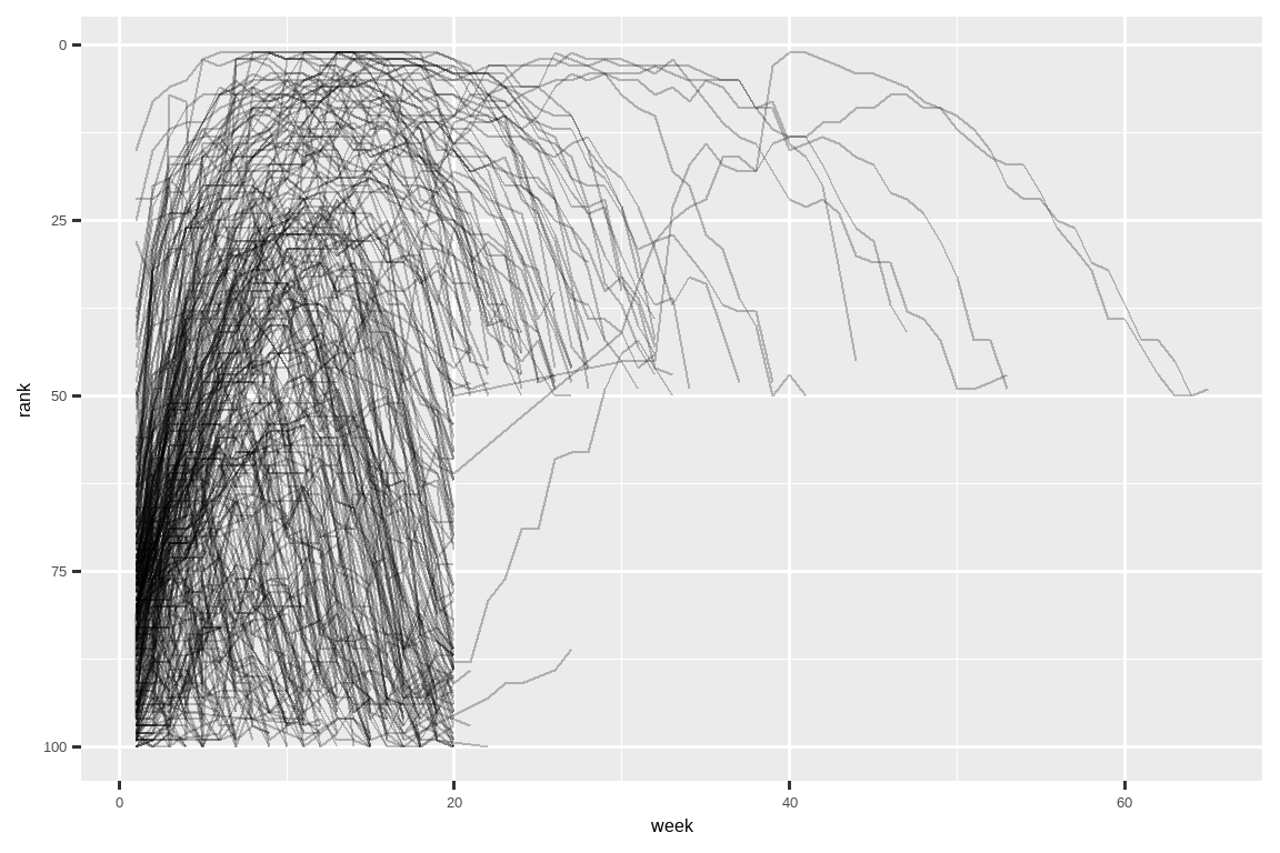

Figure 5.2: A line plot showing how the rank of a song changes over time.

5.3.2 How does pivoting work?

Now that you’ve seen how we can use pivoting to reshape our data, let’s take a little time to gain some intuition about what pivoting does to the data. Let’s start with a very simple dataset to make it easier to see what’s happening. Suppose we have three patients with ids A, B, and C, and we take two blood pressure measurements on each patient. We’ll create the data with tribble(), a handy function for constructing small tibbles by hand:
既然你已经看到了如何使用透视来重塑数据，让我们花点时间来直观地了解一下透视对数据的作用。 让我们从一个非常简单的数据集开始，以便更容易地看清发生了什么。 假设我们有三个病人，他们的 id 分别是 A、B 和 C，我们对每个病人进行了两次血压测量。 我们将使用 tribble() 创建数据，这是一个方便手动构建小型 tibble 的函数：

df <- tribble(
  ~id,  ~bp1, ~bp2,
   "A",  100,  120,
   "B",  140,  115,
   "C",  120,  125
)

We want our new dataset to have three variables: id (already exists), measurement (the column names), and value (the cell values). To achieve this, we need to pivot df longer:
我们希望新数据集有三个变量：id（已存在）、measurement（列名）和 value（单元格值）。 为了实现这一点，我们需要将 df 透视得更长：

df |> 
  pivot_longer(
    cols = bp1:bp2,
    names_to = "measurement",
    values_to = "value"
  )
#> # A tibble: 6 × 3
#>   id    measurement value
#>   <chr> <chr>       <dbl>
#> 1 A     bp1           100
#> 2 A     bp2           120
#> 3 B     bp1           140
#> 4 B     bp2           115
#> 5 C     bp1           120
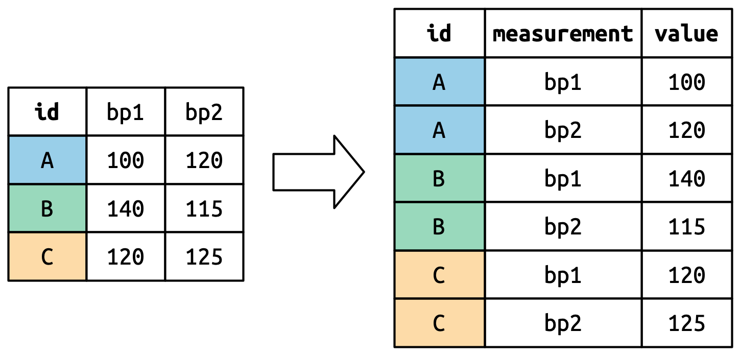
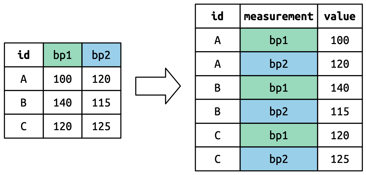
#> 6 C     bp2           125

How does the reshaping work? It’s easier to see if we think about it column by column. As shown in Figure 5.3, the values in a column that was already a variable in the original dataset (id) need to be repeated, once for each column that is pivoted.
重塑是如何工作的？ 如果我们逐列思考，会更容易理解。 如 Figure 5.3 所示，原始数据集中已经是变量的列（id）中的值需要重复，每个被透视的列重复一次。

Figure 5.3: Columns that are already variables need to be repeated, once for each column that is pivoted.

The column names become values in a new variable, whose name is defined by names_to, as shown in Figure 5.4. They need to be repeated once for each row in the original dataset.
列名成为一个新变量中的值，该新变量的名称由 names_to 定义，如 Figure 5.4 所示。 它们需要为原始数据集中的每一行重复一次。

Figure 5.4: The column names of pivoted columns become values in a new column. The values need to be repeated once for each row of the original dataset.

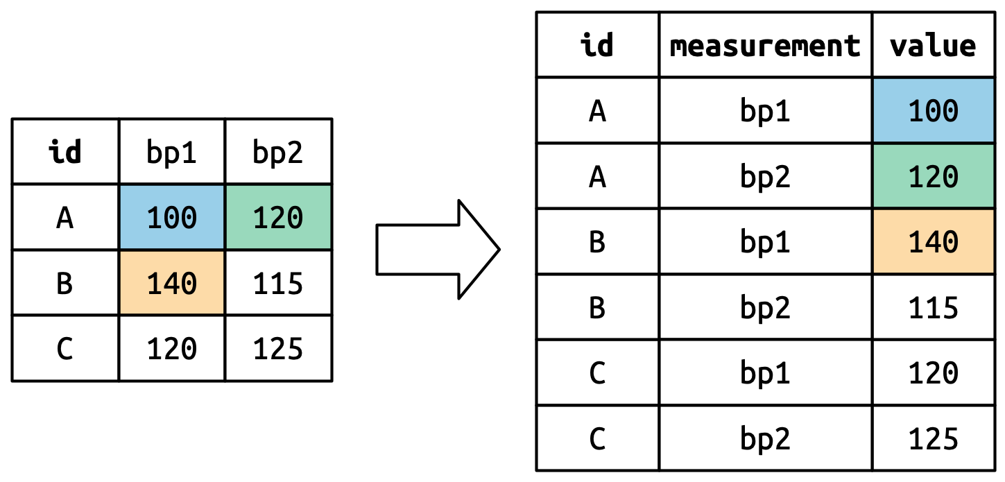
The cell values also become values in a new variable, with a name defined by values_to. They are unwound row by row. Figure 5.5 illustrates the process.
单元格的值也成为一个新变量中的值，其名称由 values_to 定义。 它们是逐行展开的。 Figure 5.5 说明了这个过程。

Figure 5.5: The number of values is preserved (not repeated), but unwound row-by-row.

5.3.3 Many variables in column names

A more challenging situation occurs when you have multiple pieces of information crammed into the column names, and you would like to store these in separate new variables. For example, take the who2 dataset, the source of table1 and friends that you saw above:
一个更具挑战性的情况是，当你有多条信息挤在列名中，而你希望将它们存储在不同的新变量中时。 例如，以 who2 数据集为例，这是你之前看到的 table1 及相关表格的来源：

who2
#> # A tibble: 7,240 × 58
#>   country      year sp_m_014 sp_m_1524 sp_m_2534 sp_m_3544 sp_m_4554
#>   <chr>       <dbl>    <dbl>     <dbl>     <dbl>     <dbl>     <dbl>
#> 1 Afghanistan  1980       NA        NA        NA        NA        NA
#> 2 Afghanistan  1981       NA        NA        NA        NA        NA
#> 3 Afghanistan  1982       NA        NA        NA        NA        NA
#> 4 Afghanistan  1983       NA        NA        NA        NA        NA
#> 5 Afghanistan  1984       NA        NA        NA        NA        NA
#> 6 Afghanistan  1985       NA        NA        NA        NA        NA
#> # ℹ 7,234 more rows
#> # ℹ 51 more variables: sp_m_5564 <dbl>, sp_m_65 <dbl>, sp_f_014 <dbl>, …

This dataset, collected by the World Health Organisation, records information about tuberculosis diagnoses. There are two columns that are already variables and are easy to interpret: country and year. They are followed by 56 columns like sp_m_014, ep_m_4554, and rel_m_3544. If you stare at these columns for long enough, you’ll notice there’s a pattern. Each column name is made up of three pieces separated by _. The first piece, sp/rel/ep, describes the method used for the diagnosis, the second piece, m/f is the gender (coded as a binary variable in this dataset), and the third piece, 014/1524/2534/3544/4554/5564/65 is the age range (014 represents 0-14, for example).
这个由世界卫生组织收集的数据集记录了关于结核病诊断的信息。 有两列已经是变量且易于解释：country 和 year。 紧随其后的是 56 个类似 sp_m_014、ep_m_4554 和 rel_m_3544 的列。 如果你盯着这些列足够长的时间，你会注意到一个模式。 每个列名由三个部分组成，用 _ 分隔。 第一部分 sp/rel/ep 描述了诊断方法，第二部分 m/f 是 gender（性别，在此数据集中编码为二元变量），第三部分 014/1524/2534/3544/4554/5564/65 是 age（年龄）范围（例如，014 代表 0-14 岁）。

So in this case we have six pieces of information recorded in who2: the country and the year (already columns); the method of diagnosis, the gender category, and the age range category (contained in the other column names); and the count of patients in that category (cell values). To organize these six pieces of information in six separate columns, we use pivot_longer() with a vector of column names for names_to and instructors for splitting the original variable names into pieces for names_sep as well as a column name for values_to:
因此，在这种情况下，我们在 who2 中记录了六条信息：国家和年份（已是列）；诊断方法、性别类别和年龄范围类别（包含在其他列名中）；以及该类别中的患者计数（单元格值）。 为了将这六条信息组织在六个独立的列中，我们使用 pivot_longer()，为 names_to 提供一个列名向量，为 names_sep 提供将原始变量名拆分成片段的指令，并为 values_to 提供一个列名：

who2 |> 
  pivot_longer(
    cols = !(country:year),
    names_to = c("diagnosis", "gender", "age"), 
    names_sep = "_",
    values_to = "count"
  )
#> # A tibble: 405,440 × 6
#>   country      year diagnosis gender age   count
#>   <chr>       <dbl> <chr>     <chr>  <chr> <dbl>
#> 1 Afghanistan  1980 sp        m      014      NA
#> 2 Afghanistan  1980 sp        m      1524     NA
#> 3 Afghanistan  1980 sp        m      2534     NA
#> 4 Afghanistan  1980 sp        m      3544     NA
#> 5 Afghanistan  1980 sp        m      4554     NA
#> 6 Afghanistan  1980 sp        m      5564     NA
#> # ℹ 405,434 more rows

An alternative to names_sep is names_pattern, which you can use to extract variables from more complicated naming scenarios, once you’ve learned about regular expressions in Chapter 15.
names_sep 的一个替代方案是 names_pattern，在你学习了 Chapter 15 中的正则表达式后，可以用它从更复杂的命名场景中提取变量。

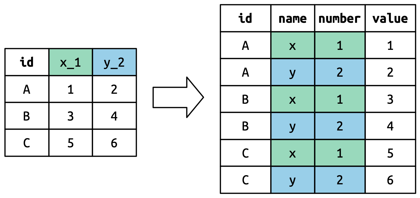
Conceptually, this is only a minor variation on the simpler case you’ve already seen. Figure 5.6 shows the basic idea: now, instead of the column names pivoting into a single column, they pivot into multiple columns. You can imagine this happening in two steps (first pivoting and then separating) but under the hood it happens in a single step because that’s faster.
从概念上讲，这只是你已经看过的简单情况的一个微小变体。 Figure 5.6 展示了基本思想：现在，列名不是透视到单个列中，而是透视到多个列中。 你可以想象这分两步发生（先透视再分离），但在底层它是一步完成的，因为这样更快。

Figure 5.6: Pivoting columns with multiple pieces of information in the names means that each column name now fills in values in multiple output columns.

5.3.4 Data and variable names in the column headers

The next step up in complexity is when the column names include a mix of variable values and variable names. For example, take the household dataset:
下一个复杂程度的提升是当列名中混合了变量值和变量名。 例如，以 household 数据集为例：

household
#> # A tibble: 5 × 5
#>   family dob_child1 dob_child2 name_child1 name_child2
#>    <int> <date>     <date>     <chr>       <chr>      
#> 1      1 1998-11-26 2000-01-29 Susan       Jose       
#> 2      2 1996-06-22 NA         Mark        <NA>       
#> 3      3 2002-07-11 2004-04-05 Sam         Seth       
#> 4      4 2004-10-10 2009-08-27 Craig       Khai       
#> 5      5 2000-12-05 2005-02-28 Parker      Gracie

This dataset contains data about five families, with the names and dates of birth of up to two children. The new challenge in this dataset is that the column names contain the names of two variables (dob, name) and the values of another (child, with values 1 or 2). To solve this problem we again need to supply a vector to names_to but this time we use the special ".value" sentinel; this isn’t the name of a variable but a unique value that tells pivot_longer() to do something different. This overrides the usual values_to argument to use the first component of the pivoted column name as a variable name in the output.
该数据集包含五个家庭的数据，其中包含最多两个孩子的姓名和出生日期。 这个数据集中的新挑战是，列名包含了两个变量的名称（dob、name）和另一个变量的值（child，值为 1 或 2）。 要解决这个问题，我们再次需要向 names_to 提供一个向量，但这次我们使用特殊的 ".value" 标记；这不是一个变量名，而是一个特殊的值，告诉 pivot_longer() 做一些不同的事情。 这会覆盖通常的 values_to 参数，转而使用被透视列名的第一个组成部分作为输出中的变量名。

household |> 
  pivot_longer(
    cols = !family, 
    names_to = c(".value", "child"), 
    names_sep = "_", 
    values_drop_na = TRUE
  )
#> # A tibble: 9 × 4
#>   family child  dob        name 
#>    <int> <chr>  <date>     <chr>
#> 1      1 child1 1998-11-26 Susan
#> 2      1 child2 2000-01-29 Jose 
#> 3      2 child1 1996-06-22 Mark 
#> 4      3 child1 2002-07-11 Sam  
#> 5      3 child2 2004-04-05 Seth 
#> 6      4 child1 2004-10-10 Craig
#> # ℹ 3 more rows

We again use values_drop_na = TRUE, since the shape of the input forces the creation of explicit missing variables (e.g., for families with only one child).
我们再次使用 values_drop_na = TRUE，因为输入的形状强制创建了显式的缺失变量（例如，对于只有一个孩子的家庭）。

Figure 5.7 illustrates the basic idea with a simpler example. When you use ".value" in names_to, the column names in the input contribute to both values and variable names in the output.
Figure 5.7 用一个更简单的例子阐述了基本思想。 当你在 names_to 中使用 ".value" 时，输入中的列名同时贡献于输出中的值和变量名。

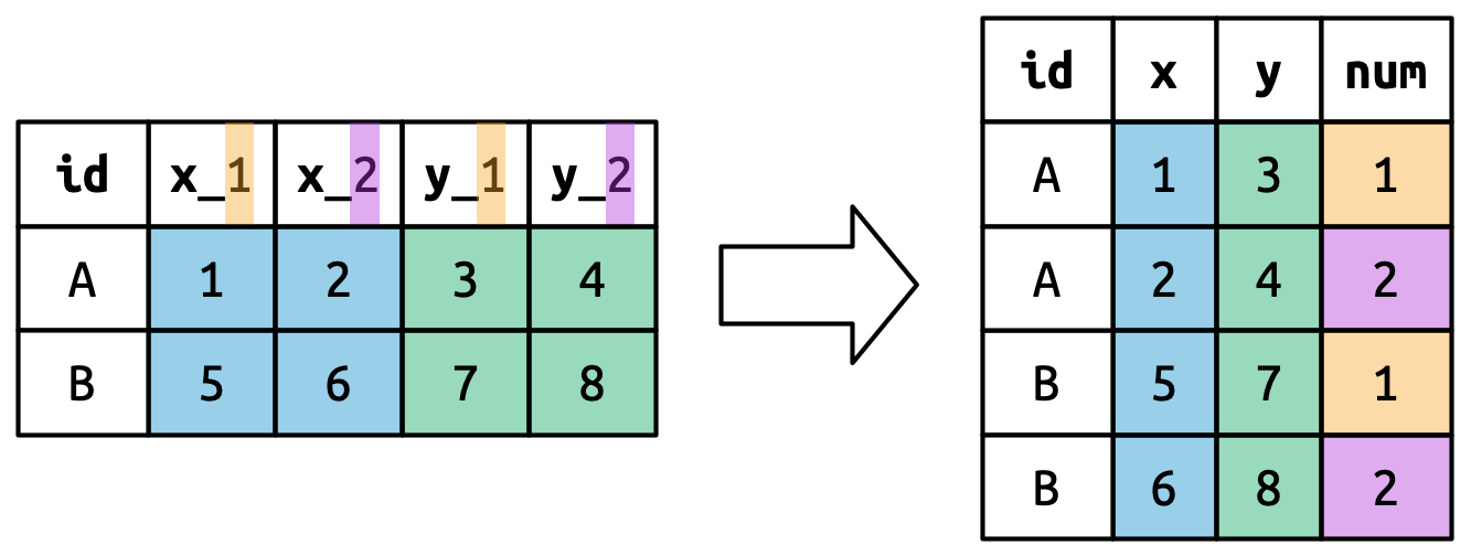
Figure 5.7: Pivoting with names_to = c(".value", "num") splits the column names into two components: the first part determines the output column name (x or y), and the second part determines the value of the num column.

5.4 Widening data

So far we’ve used pivot_longer() to solve the common class of problems where values have ended up in column names. Next we’ll pivot (HA HA) to pivot_wider(), which makes datasets wider by increasing columns and reducing rows and helps when one observation is spread across multiple rows. This seems to arise less commonly in the wild, but it does seem to crop up a lot when dealing with governmental data.
到目前为止，我们已经使用 pivot_longer() 解决了值最终出现在列名中的一类常见问题。 接下来，我们将转向（哈哈，一语双关）pivot_wider()，它通过增加列数和减少行数使数据集变宽，并在一个观测分布在多行时提供帮助。 这种情况在现实世界中似乎不那么常见，但在处理政府数据时却经常出现。

We’ll start by looking at cms_patient_experience, a dataset from the Centers of Medicare and Medicaid services that collects data about patient experiences:
我们将从 cms_patient_experience 数据集开始，这是一个来自医疗保险和医疗补助服务中心 (Centers of Medicare and Medicaid services) 的数据集，收集了关于患者体验的数据：

cms_patient_experience
#> # A tibble: 500 × 5
#>   org_pac_id org_nm                     measure_cd   measure_title   prf_rate
#>   <chr>      <chr>                      <chr>        <chr>              <dbl>
#> 1 0446157747 USC CARE MEDICAL GROUP INC CAHPS_GRP_1  CAHPS for MIPS…       63
#> 2 0446157747 USC CARE MEDICAL GROUP INC CAHPS_GRP_2  CAHPS for MIPS…       87
#> 3 0446157747 USC CARE MEDICAL GROUP INC CAHPS_GRP_3  CAHPS for MIPS…       86
#> 4 0446157747 USC CARE MEDICAL GROUP INC CAHPS_GRP_5  CAHPS for MIPS…       57
#> 5 0446157747 USC CARE MEDICAL GROUP INC CAHPS_GRP_8  CAHPS for MIPS…       85
#> 6 0446157747 USC CARE MEDICAL GROUP INC CAHPS_GRP_12 CAHPS for MIPS…       24
#> # ℹ 494 more rows

The core unit being studied is an organization, but each organization is spread across six rows, with one row for each measurement taken in the survey organization. We can see the complete set of values for measure_cd and measure_title by using distinct():
研究的核心单位是一个组织，但每个组织的数据分布在六行中，每一行对应于该调查组织进行的一项测量。 我们可以使用 distinct() 查看 measure_cd 和 measure_title 的完整值集合：

cms_patient_experience |> 
  distinct(measure_cd, measure_title)
#> # A tibble: 6 × 2
#>   measure_cd   measure_title                                                 
#>   <chr>        <chr>                                                         
#> 1 CAHPS_GRP_1  CAHPS for MIPS SSM: Getting Timely Care, Appointments, and In…
#> 2 CAHPS_GRP_2  CAHPS for MIPS SSM: How Well Providers Communicate            
#> 3 CAHPS_GRP_3  CAHPS for MIPS SSM: Patient's Rating of Provider              
#> 4 CAHPS_GRP_5  CAHPS for MIPS SSM: Health Promotion and Education            
#> 5 CAHPS_GRP_8  CAHPS for MIPS SSM: Courteous and Helpful Office Staff        
#> 6 CAHPS_GRP_12 CAHPS for MIPS SSM: Stewardship of Patient Resources

Neither of these columns will make particularly great variable names: measure_cd doesn’t hint at the meaning of the variable and measure_title is a long sentence containing spaces. We’ll use measure_cd as the source for our new column names for now, but in a real analysis you might want to create your own variable names that are both short and meaningful.
这两列都不能成为特别好的变量名：measure_cd 没有暗示变量的含义，而 measure_title 是一个包含空格的长句子。 我们暂时使用 measure_cd 作为新列名的来源，但在实际分析中，你可能希望创建既简短又有意义的自己的变量名。

pivot_wider() has the opposite interface to pivot_longer(): instead of choosing new column names, we need to provide the existing columns that define the values (values_from) and the column name (names_from):
pivot_wider() 的接口与 pivot_longer() 相反：我们不是选择新的列名，而是需要提供定义值的现有列 (values_from) 和定义列名的列 (names_from)：

cms_patient_experience |> 
  pivot_wider(
    names_from = measure_cd,
    values_from = prf_rate
  )
#> # A tibble: 500 × 9
#>   org_pac_id org_nm                   measure_title   CAHPS_GRP_1 CAHPS_GRP_2
#>   <chr>      <chr>                    <chr>                 <dbl>       <dbl>
#> 1 0446157747 USC CARE MEDICAL GROUP … CAHPS for MIPS…          63          NA
#> 2 0446157747 USC CARE MEDICAL GROUP … CAHPS for MIPS…          NA          87
#> 3 0446157747 USC CARE MEDICAL GROUP … CAHPS for MIPS…          NA          NA
#> 4 0446157747 USC CARE MEDICAL GROUP … CAHPS for MIPS…          NA          NA
#> 5 0446157747 USC CARE MEDICAL GROUP … CAHPS for MIPS…          NA          NA
#> 6 0446157747 USC CARE MEDICAL GROUP … CAHPS for MIPS…          NA          NA
#> # ℹ 494 more rows
#> # ℹ 4 more variables: CAHPS_GRP_3 <dbl>, CAHPS_GRP_5 <dbl>, …

The output doesn’t look quite right; we still seem to have multiple rows for each organization. That’s because, we also need to tell pivot_wider() which column or columns have values that uniquely identify each row; in this case those are the variables starting with "org":
输出看起来不太对；我们似乎每个组织仍然有多行。 这是因为，我们还需要告诉 pivot_wider() 哪个或哪些列的值可以唯一标识每一行；在这种情况下，这些是以 "org" 开头的变量：

cms_patient_experience |> 
  pivot_wider(
    id_cols = starts_with("org"),
    names_from = measure_cd,
    values_from = prf_rate
  )
#> # A tibble: 95 × 8
#>   org_pac_id org_nm           CAHPS_GRP_1 CAHPS_GRP_2 CAHPS_GRP_3 CAHPS_GRP_5
#>   <chr>      <chr>                  <dbl>       <dbl>       <dbl>       <dbl>
#> 1 0446157747 USC CARE MEDICA…          63          87          86          57
#> 2 0446162697 ASSOCIATION OF …          59          85          83          63
#> 3 0547164295 BEAVER MEDICAL …          49          NA          75          44
#> 4 0749333730 CAPE PHYSICIANS…          67          84          85          65
#> 5 0840104360 ALLIANCE PHYSIC…          66          87          87          64
#> 6 0840109864 REX HOSPITAL INC          73          87          84          67
#> # ℹ 89 more rows
#> # ℹ 2 more variables: CAHPS_GRP_8 <dbl>, CAHPS_GRP_12 <dbl>

This gives us the output that we’re looking for.
这就得到了我们想要的结果。

5.4.1 How does pivot_wider() work?

To understand how pivot_wider() works, let’s again start with a very simple dataset. This time we have two patients with ids A and B, we have three blood pressure measurements on patient A and two on patient B:
为了理解 pivot_wider() 的工作原理，我们再次从一个非常简单的数据集开始。 这次我们有两个病人，ID 分别为 A 和 B，我们对病人 A 进行了三次血压测量，对病人 B 进行了两次：

df <- tribble(
  ~id, ~measurement, ~value,
  "A",        "bp1",    100,
  "B",        "bp1",    140,
  "B",        "bp2",    115, 
  "A",        "bp2",    120,
  "A",        "bp3",    105
)

We’ll take the values from the value column and the names from the measurement column:
我们将从 value 列中获取值，从 measurement 列中获取名称：

df |> 
  pivot_wider(
    names_from = measurement,
    values_from = value
  )
#> # A tibble: 2 × 4
#>   id      bp1   bp2   bp3
#>   <chr> <dbl> <dbl> <dbl>
#> 1 A       100   120   105
#> 2 B       140   115    NA

To begin the process pivot_wider() needs to first figure out what will go in the rows and columns. The new column names will be the unique values of measurement.
要开始这个过程，pivot_wider() 首先需要确定行和列的内容。 新的列名将是 measurement 的唯一值。

df |> 
  distinct(measurement) |> 
  pull()
#> [1] "bp1" "bp2" "bp3"

By default, the rows in the output are determined by all the variables that aren’t going into the new names or values. These are called the id_cols. Here there is only one column, but in general there can be any number.
默认情况下，输出中的行由所有不用于新名称或值的变量决定。 这些被称为 id_cols。 这里只有一个列，但通常可以有任意数量的列。

df |> 
  select(-measurement, -value) |> 
  distinct()
#> # A tibble: 2 × 1
#>   id   
#>   <chr>
#> 1 A    
#> 2 B

pivot_wider() then combines these results to generate an empty data frame:
然后，pivot_wider() 结合这些结果生成一个空的数据框：

df |> 
  select(-measurement, -value) |> 
  distinct() |> 
  mutate(x = NA, y = NA, z = NA)
#> # A tibble: 2 × 4
#>   id    x     y     z    
#>   <chr> <lgl> <lgl> <lgl>
#> 1 A     NA    NA    NA   
#> 2 B     NA    NA    NA

It then fills in all the missing values using the data in the input. In this case, not every cell in the output has a corresponding value in the input as there’s no third blood pressure measurement for patient B, so that cell remains missing. We’ll come back to this idea that pivot_wider() can “make” missing values in Chapter 18.
然后，它使用输入中的数据填充所有缺失值。 在这种情况下，输出中的并非每个单元格在输入中都有对应的值，因为病人 B 没有第三次血压测量值，所以该单元格保持缺失状态。 我们将在 Chapter 18 中再次讨论 pivot_wider() 可以“制造”缺失值的这个概念。

You might also wonder what happens if there are multiple rows in the input that correspond to one cell in the output. The example below has two rows that correspond to id “A” and measurement “bp1”:
你可能还会想，如果输入中有多个行对应于输出中的一个单元格，会发生什么。 下面的例子中有两行对应 id “A” 和 measurement “bp1”：

df <- tribble(
  ~id, ~measurement, ~value,
  "A",        "bp1",    100,
  "A",        "bp1",    102,
  "A",        "bp2",    120,
  "B",        "bp1",    140, 
  "B",        "bp2",    115
)

If we attempt to pivot this we get an output that contains list-columns, which you’ll learn more about in Chapter 23:
如果我们尝试对此进行透视，我们会得到一个包含列表列（list-columns）的输出，你将在 Chapter 23 中学到更多相关内容：

df |>
  pivot_wider(
    names_from = measurement,
    values_from = value
  )
#> Warning: Values from `value` are not uniquely identified; output will contain
#> list-cols.
#> • Use `values_fn = list` to suppress this warning.
#> • Use `values_fn = {summary_fun}` to summarise duplicates.
#> • Use the following dplyr code to identify duplicates.
#>   {data} |>
#>   dplyr::summarise(n = dplyr::n(), .by = c(id, measurement)) |>
#>   dplyr::filter(n > 1L)
#> # A tibble: 2 × 3
#>   id    bp1       bp2      
#>   <chr> <list>    <list>   
#> 1 A     <dbl [2]> <dbl [1]>
#> 2 B     <dbl [1]> <dbl [1]>

Since you don’t know how to work with this sort of data yet, you’ll want to follow the hint in the warning to figure out where the problem is:
由于你还不知道如何处理这类数据，你可能需要遵循警告中的提示来找出问题所在：

df |> 
  group_by(id, measurement) |> 
  summarize(n = n(), .groups = "drop") |> 
  filter(n > 1)
#> # A tibble: 1 × 3
#>   id    measurement     n
#>   <chr> <chr>       <int>
#> 1 A     bp1             2

It’s then up to you to figure out what’s gone wrong with your data and either repair the underlying damage or use your grouping and summarizing skills to ensure that each combination of row and column values only has a single row.
接下来就由你来找出数据中出了什么问题，要么修复潜在的损坏，要么利用你的分组和汇总技能，确保行和列值的每个组合只有一个单行。

5.5 Summary

In this chapter you learned about tidy data: data that has variables in columns and observations in rows. Tidy data makes working in the tidyverse easier, because it’s a consistent structure understood by most functions, the main challenge is transforming the data from whatever structure you receive it in to a tidy format. To that end, you learned about pivot_longer() and pivot_wider() which allow you to tidy up many untidy datasets. The examples we presented here are a selection of those from vignette("pivot", package = "tidyr"), so if you encounter a problem that this chapter doesn’t help you with, that vignette is a good place to try next.
在本章中，你学习了整洁数据：即变量在列、观测在行的数据。 整洁数据使得在 tidyverse 中工作更加容易，因为它是一个被大多数函数所理解的一致性结构，主要的挑战在于将你收到的任何结构的数据转换为整洁格式。 为此，你学习了 pivot_longer() 和 pivot_wider()，它们可以让你整理许多不整洁的数据集。 我们在这里展示的例子选自 vignette("pivot", package = "tidyr")，所以如果你遇到本章无法解决的问题，那篇小品文是一个很好的下一步尝试。

Another challenge is that, for a given dataset, it can be impossible to label the longer or the wider version as the “tidy” one. This is partly a reflection of our definition of tidy data, where we said tidy data has one variable in each column, but we didn’t actually define what a variable is (and it’s surprisingly hard to do so). It’s totally fine to be pragmatic and to say a variable is whatever makes your analysis easiest. So if you’re stuck figuring out how to do some computation, consider switching up the organisation of your data; don’t be afraid to untidy, transform, and re-tidy as needed!
另一个挑战是，对于给定的数据集，可能无法将长格式或宽格式版本标记为“整洁”的版本。 这部分反映了我们对整洁数据的定义，我们说整洁数据每列有一个变量，但我们实际上没有定义什么是变量（而且令人惊讶的是，这很难做到）。 采取务实的态度是完全可以的，可以说变量就是任何使你的分析最容易的东西。 所以，如果你在计算上遇到困难，可以考虑改变数据的组织方式；不要害怕按需进行非整洁化、转换和重新整理！

If you enjoyed this chapter and want to learn more about the underlying theory, you can learn more about the history and theoretical underpinnings in the Tidy Data paper published in the Journal of Statistical Software.
如果你喜欢这一章并想了解更多关于其背后理论的知识，你可以在发表于《统计软件杂志》(Journal of Statistical Software) 的 Tidy Data 论文中了解更多关于其历史和理论基础的内容。

Now that you’re writing a substantial amount of R code, it’s time to learn more about organizing your code into files and directories. In the next chapter, you’ll learn all about the advantages of scripts and projects, and some of the many tools that they provide to make your life easier.
现在你已经编写了大量的 R 代码，是时候学习更多关于将代码组织到文件和目录中的知识了。 在下一章中，你将学习脚本和项目的所有优点，以及它们为使你的生活更轻松而提供的许多工具。

---

1. The song will be included as long as it was in the top 100 at some point in 2000, and is tracked for up to 72 weeks after it appears.

2. We’ll come back to this idea in Chapter 18.