library(nycflights13)
library(tidyverse)
#> ── Attaching core tidyverse packages ───────────────────── tidyverse 2.0.0 ──
#> ✔ dplyr     1.1.4     ✔ readr     2.1.5
#> ✔ forcats   1.0.0     ✔ stringr   1.5.1
#> ✔ ggplot2   3.5.2     ✔ tibble    3.3.0
#> ✔ lubridate 1.9.4     ✔ tidyr     1.3.1
#> ✔ purrr     1.0.4
#> ── Conflicts ─────────────────────────────────────── tidyverse_conflicts() ──
#> ✖ dplyr::filter() masks stats::filter()
#> ✖ dplyr::lag()    masks stats::lag()
#> ℹ Use the conflicted package (<http://conflicted.r-lib.org/>) to force all conflicts to become errors3 数据转换
3.1 引言
可视化是产生洞见的重要工具,但你很少能得到完全符合你需求的、可以直接用来制作你想要的图表的数据形式。通常,你需要创建一些新的变量或摘要来用数据回答你的问题,或者你可能只是想重命名变量或重新排序观测值,以便让数据更容易处理。在本章中,你将学习如何做到所有这些(以及更多!),本章将向你介绍如何使用 dplyr 包和一个关于 2013 年从纽约市起飞的航班的新数据集来进行数据转换。
本章的目标是让你对所有用于转换数据框的关键工具有一个全面的了解。我们将从操作数据框的行和列的函数开始,然后回过头来更多地讨论管道 (pipe),这是一个用于组合动词的重要工具。接着,我们将介绍处理分组的能力。本章最后会有一个案例研究,展示这些函数的实际应用。在后面的章节中,当我们开始深入研究特定类型的数据(例如,数字、字符串、日期)时,我们将更详细地回顾这些函数。
3.1.1 先决条件
在本章中,我们将重点关注 dplyr 包,它是 tidyverse 的另一个核心成员。我们将使用 nycflights13 包中的数据来说明关键思想,并使用 ggplot2 来帮助我们理解数据。
请仔细注意加载 tidyverse 时打印出的冲突信息。它告诉你 dplyr 覆盖了 R 基础包中的一些函数。如果你在加载 dplyr 后想使用这些函数的基础版本,你需要使用它们的全名:stats::filter() 和 stats::lag()。到目前为止,我们大多忽略了函数来自哪个包,因为这通常不重要。然而,知道包可以帮助你找到帮助和相关函数,所以当我们需要精确说明一个函数来自哪个包时,我们将使用与 R 相同的语法:packagename::functionname()。
3.1.2 nycflights13
为了探索基本的 dplyr 动词,我们将使用 nycflights13::flights。这个数据集包含了 2013 年从纽约市起飞的所有 336,776 个航班。数据来自美国交通统计局,并在 ?flights 中有文档说明。
flights
#> # A tibble: 336,776 × 19
#>    year month   day dep_time sched_dep_time dep_delay arr_time sched_arr_time
#>   <int> <int> <int>    <int>          <int>     <dbl>    <int>          <int>
#> 1  2013     1     1      517            515         2      830            819
#> 2  2013     1     1      533            529         4      850            830
#> 3  2013     1     1      542            540         2      923            850
#> 4  2013     1     1      544            545        -1     1004           1022
#> 5  2013     1     1      554            600        -6      812            837
#> 6  2013     1     1      554            558        -4      740            728
#> # ℹ 336,770 more rows
#> # ℹ 11 more variables: arr_delay <dbl>, carrier <chr>, flight <int>, …
flights 是一个 tibble,这是 tidyverse 使用的一种特殊类型的数据框,以避免一些常见的陷阱。tibble 和数据框之间最重要的区别是 tibble 的打印方式;它们专为大型数据集设计,因此只显示前几行和能在一个屏幕上容纳的列。有几种方法可以查看所有内容。如果你正在使用 RStudio,最方便的可能是 View(flights),它会打开一个可交互、可滚动和可筛选的视图。否则你可以使用 print(flights, width = Inf) 来显示所有列,或者使用 glimpse():
glimpse(flights)
#> Rows: 336,776
#> Columns: 19
#> $ year           <int> 2013, 2013, 2013, 2013, 2013, 2013, 2013, 2013, 2013…
#> $ month          <int> 1, 1, 1, 1, 1, 1, 1, 1, 1, 1, 1, 1, 1, 1, 1, 1, 1, 1…
#> $ day            <int> 1, 1, 1, 1, 1, 1, 1, 1, 1, 1, 1, 1, 1, 1, 1, 1, 1, 1…
#> $ dep_time       <int> 517, 533, 542, 544, 554, 554, 555, 557, 557, 558, 55…
#> $ sched_dep_time <int> 515, 529, 540, 545, 600, 558, 600, 600, 600, 600, 60…
#> $ dep_delay      <dbl> 2, 4, 2, -1, -6, -4, -5, -3, -3, -2, -2, -2, -2, -2,…
#> $ arr_time       <int> 830, 850, 923, 1004, 812, 740, 913, 709, 838, 753, 8…
#> $ sched_arr_time <int> 819, 830, 850, 1022, 837, 728, 854, 723, 846, 745, 8…
#> $ arr_delay      <dbl> 11, 20, 33, -18, -25, 12, 19, -14, -8, 8, -2, -3, 7,…
#> $ carrier        <chr> "UA", "UA", "AA", "B6", "DL", "UA", "B6", "EV", "B6"…
#> $ flight         <int> 1545, 1714, 1141, 725, 461, 1696, 507, 5708, 79, 301…
#> $ tailnum        <chr> "N14228", "N24211", "N619AA", "N804JB", "N668DN", "N…
#> $ origin         <chr> "EWR", "LGA", "JFK", "JFK", "LGA", "EWR", "EWR", "LG…
#> $ dest           <chr> "IAH", "IAH", "MIA", "BQN", "ATL", "ORD", "FLL", "IA…
#> $ air_time       <dbl> 227, 227, 160, 183, 116, 150, 158, 53, 140, 138, 149…
#> $ distance       <dbl> 1400, 1416, 1089, 1576, 762, 719, 1065, 229, 944, 73…
#> $ hour           <dbl> 5, 5, 5, 5, 6, 5, 6, 6, 6, 6, 6, 6, 6, 6, 6, 5, 6, 6…
#> $ minute         <dbl> 15, 29, 40, 45, 0, 58, 0, 0, 0, 0, 0, 0, 0, 0, 0, 59…
#> $ time_hour <dttm> 2013-01-01 05:00:00, 2013-01-01 05:00:00, 2013-01-0…在这两种视图中,变量名后面都跟着缩写,告诉你每个变量的类型:<int> 是整数 (integer) 的缩写,<dbl> 是双精度浮点数 (double)(也就是实数)的缩写,<chr> 是字符 (character)(也就是字符串)的缩写,<dttm> 是日期时间 (date-time) 的缩写。这些都很重要,因为你可以对一列执行的操作在很大程度上取决于它的“类型”。
3.1.3 dplyr 基础
你即将学习主要的 dplyr 动词(函数),它们将使你能够解决绝大多数数据操作挑战。但在我们讨论它们各自的差异之前,值得说明一下它们的共同点:
第一个参数总是一个数据框。
后续的参数通常使用变量名(不带引号)来描述要操作的列。
输出总是一个新的数据框。
因为每个动词都只做好一件事,所以解决复杂问题通常需要组合多个动词,我们将使用管道 |> 来实现这一点。我们将在 Section 3.4 中更多地讨论管道,但简而言之,管道将其左侧的内容传递给右侧的函数,因此 x |> f(y) 等同于 f(x, y),而 x |> f(y) |> g(z) 等同于 g(f(x, y), z)。管道最简单的发音方式是“然后 (then)”。这使得即使你还没有学习细节,也能对以下代码有一个大致的了解:
dplyr 的动词根据它们操作的对象分为四组:行 (rows)、列 (columns)、组 (groups) 或表 (tables)。在接下来的部分中,你将学习针对行、列和组的最重要的动词。然后,我们将在 Chapter 19 中回到处理表的连接动词。让我们开始吧!
3.2 行
操作数据集行的最重要的动词是 filter() 和 arrange()。filter() 可以在不改变行顺序的情况下改变哪些行存在,而 arrange() 可以在不改变哪些行存在的情况下改变行的顺序。这两个函数都只影响行,列保持不变。我们还将讨论 distinct(),它能找到具有唯一值的行。与 arrange() 和 filter() 不同,它也可以选择性地修改列。
3.2.1 filter()
filter() 允许你根据列的值保留行1。第一个参数是数据框。第二个及后续参数是保留行必须满足的条件。例如,我们可以找到所有晚点超过 120 分钟(两小时)起飞的航班:
flights |>
    filter(dep_delay > 120)
#> # A tibble: 9,723 × 19
#>    year month   day dep_time sched_dep_time dep_delay arr_time sched_arr_time
#>   <int> <int> <int>    <int>          <int>     <dbl>    <int>          <int>
#> 1  2013     1     1      848           1835       853     1001           1950
#> 2  2013     1     1      957            733       144     1056            853
#> 3  2013     1     1     1114            900       134     1447           1222
#> 4  2013     1     1     1540           1338       122     2020           1825
#> 5  2013     1     1     1815           1325       290     2120           1542
#> 6  2013     1     1     1842           1422       260     1958           1535
#> # ℹ 9,717 more rows
#> # ℹ 11 more variables: arr_delay <dbl>, carrier <chr>, flight <int>, …
除了 >(大于),你还可以使用 >=(大于或等于)、<(小于)、<=(小于或等于)、==(等于)和 !=(不等于)。你还可以用 & 或 , 组合条件来表示“与”(检查两个条件),或用 | 来表示“或”(检查任一条件):
# 1 月 1 日起飞的航班
flights |>
    filter(month == 1 & day == 1)
#> # A tibble: 842 × 19
#>    year month   day dep_time sched_dep_time dep_delay arr_time sched_arr_time
#>   <int> <int> <int>    <int>          <int>     <dbl>    <int>          <int>
#> 1  2013     1     1      517            515         2      830            819
#> 2  2013     1     1      533            529         4      850            830
#> 3  2013     1     1      542            540         2      923            850
#> 4  2013     1     1      544            545        -1     1004           1022
#> 5  2013     1     1      554            600        -6      812            837
#> 6  2013     1     1      554            558        -4      740            728
#> # ℹ 836 more rows
#> # ℹ 11 more variables: arr_delay <dbl>, carrier <chr>, flight <int>, …

# 1 月或 2 月起飞的航班
flights |>
    filter(month == 1 | month == 2)
#> # A tibble: 51,955 × 19
#>    year month   day dep_time sched_dep_time dep_delay arr_time sched_arr_time
#>   <int> <int> <int>    <int>          <int>     <dbl>    <int>          <int>
#> 1  2013     1     1      517            515         2      830            819
#> 2  2013     1     1      533            529         4      850            830
#> 3  2013     1     1      542            540         2      923            850
#> 4  2013     1     1      544            545        -1     1004           1022
#> 5  2013     1     1      554            600        -6      812            837
#> 6  2013     1     1      554            558        -4      740            728
#> # ℹ 51,949 more rows
#> # ℹ 11 more variables: arr_delay <dbl>, carrier <chr>, flight <int>, …
当你组合 | 和 == 时,有一个很有用的快捷方式:%in%。它会保留变量等于右侧值之一的行:
# 一种更短的方式来选择 1 月或 2 月起飞的航班
flights |>
    filter(month %in% c(1, 2))
#> # A tibble: 51,955 × 19
#>    year month   day dep_time sched_dep_time dep_delay arr_time sched_arr_time
#>   <int> <int> <int>    <int>          <int>     <dbl>    <int>          <int>
#> 1  2013     1     1      517            515         2      830            819
#> 2  2013     1     1      533            529         4      850            830
#> 3  2013     1     1      542            540         2      923            850
#> 4  2013     1     1      544            545        -1     1004           1022
#> 5  2013     1     1      554            600        -6      812            837
#> 6  2013     1     1      554            558        -4      740            728
#> # ℹ 51,949 more rows
#> # ℹ 11 more variables: arr_delay <dbl>, carrier <chr>, flight <int>, …
我们将在 Chapter 12 中更详细地回到这些比较和逻辑运算符。
当你运行 filter() 时,dplyr 会执行筛选操作,创建一个新的数据框,然后打印它。它不会修改现有的 flights 数据集,因为 dplyr 函数从不修改它们的输入。要保存结果,你需要使用赋值运算符 <-:
jan1 <- flights |>
    filter(month == 1 & day == 1)
3.2.2 常见错误
当你刚开始使用 R 时,最容易犯的错误是在测试相等性时使用 = 而不是 ==。filter() 会在这种情况下提醒你:
flights |>
    filter(month = 1)
#> Error in `filter()`:
#> ! We detected a named input.
#> ℹ This usually means that you've used `=` instead of `==`.
#> ℹ Did you mean `month == 1`?
另一个错误是你像在英语中那样写“或”语句:
flights |>
    filter(month == 1 | 2)
这在某种意义上是“有效”的,因为它不会抛出错误,但它没有做你想要的事情,因为 | 首先检查条件 month == 1,然后检查条件 2,这不是一个合理的检查条件。我们将在 Section 12.3.2 中学习更多关于这里发生了什么以及为什么会这样。
3.2.3 arrange()
arrange() 根据列的值改变行的顺序。它接受一个数据框和一组列名(或更复杂的表达式)作为排序依据。如果你提供多个列名,每个额外的列将用于打破前一列值中的平局。例如,以下代码按出发时间排序,该时间分布在四列中。我们首先得到最早的年份,然后在一年内,最早的月份,依此类推。
flights |>
    arrange(year, month, day, dep_time)
#> # A tibble: 336,776 × 19
#>    year month   day dep_time sched_dep_time dep_delay arr_time sched_arr_time
#>   <int> <int> <int>    <int>          <int>     <dbl>    <int>          <int>
#> 1  2013     1     1      517            515         2      830            819
#> 2  2013     1     1      533            529         4      850            830
#> 3  2013     1     1      542            540         2      923            850
#> 4  2013     1     1      544            545        -1     1004           1022
#> 5  2013     1     1      554            600        -6      812            837
#> 6  2013     1     1      554            558        -4      740            728
#> # ℹ 336,770 more rows
#> # ℹ 11 more variables: arr_delay <dbl>, carrier <chr>, flight <int>, …
你可以在 arrange() 内部对一列使用 desc(),以按该列的降序(从大到小)重新排序数据框。例如,这段代码按延误时间从多到少对航班进行排序:
flights |>
    arrange(desc(dep_delay))
#> # A tibble: 336,776 × 19
#>    year month   day dep_time sched_dep_time dep_delay arr_time sched_arr_time
#>   <int> <int> <int>    <int>          <int>     <dbl>    <int>          <int>
#> 1  2013     1     9      641            900      1301     1242           1530
#> 2  2013     6    15     1432           1935      1137     1607           2120
#> 3  2013     1    10     1121           1635      1126     1239           1810
#> 4  2013     9    20     1139           1845      1014     1457           2210
#> 5  2013     7    22      845           1600      1005     1044           1815
#> 6  2013     4    10     1100           1900       960     1342           2211
#> # ℹ 336,770 more rows
#> # ℹ 11 more variables: arr_delay <dbl>, carrier <chr>, flight <int>, …
注意行数没有改变——我们只是在排列数据,而不是筛选数据。
3.2.4 distinct()
distinct() 找到数据集中的所有唯一行,所以从技术上讲,它主要操作行。然而,大多数时候,你会想要一些变量的独特组合,所以你也可以选择性地提供列名:
# 如果有的话,移除重复的行
flights |>
    distinct()
#> # A tibble: 336,776 × 19
#>    year month   day dep_time sched_dep_time dep_delay arr_time sched_arr_time
#>   <int> <int> <int>    <int>          <int>     <dbl>    <int>          <int>
#> 1  2013     1     1      517            515         2      830            819
#> 2  2013     1     1      533            529         4      850            830
#> 3  2013     1     1      542            540         2      923            850
#> 4  2013     1     1      544            545        -1     1004           1022
#> 5  2013     1     1      554            600        -6      812            837
#> 6  2013     1     1      554            558        -4      740            728
#> # ℹ 336,770 more rows
#> # ℹ 11 more variables: arr_delay <dbl>, carrier <chr>, flight <int>, …

# 找到所有唯一的出发地和目的地对
flights |>
    distinct(origin, dest)
#> # A tibble: 224 × 2
#>   origin dest
#>   <chr>  <chr>
#> 1 EWR    IAH
#> 2 LGA    IAH
#> 3 JFK    MIA
#> 4 JFK    BQN
#> 5 LGA    ATL
#> 6 EWR    ORD
#> # ℹ 218 more rows
另外,如果你想在筛选唯一行时保留其他列,你可以使用 .keep_all = TRUE 选项。
flights |>
    distinct(origin, dest, .keep_all = TRUE)
#> # A tibble: 224 × 19
#>    year month   day dep_time sched_dep_time dep_delay arr_time sched_arr_time
#>   <int> <int> <int>    <int>          <int>     <dbl>    <int>          <int>
#> 1  2013     1     1      517            515         2      830            819
#> 2  2013     1     1      533            529         4      850            830
#> 3  2013     1     1      542            540         2      923            850
#> 4  2013     1     1      544            545        -1     1004           1022
#> 5  2013     1     1      554            600        -6      812            837
#> 6  2013     1     1      554            558        -4      740            728
#> # ℹ 218 more rows
#> # ℹ 11 more variables: arr_delay <dbl>, carrier <chr>, flight <int>, …
所有这些不同的航班都在 1 月 1 日并非巧合:distinct() 会找到数据集中唯一行的第一次出现,并丢弃其余的。
如果你想找到出现的次数,最好将 distinct() 换成 count()。通过 sort = TRUE 参数,你可以按出现次数的降序排列它们。你将在 Section 13.3 中学到更多关于 count 的知识。
flights |>
    count(origin, dest, sort = TRUE)
#> # A tibble: 224 × 3
#>   origin dest      n
#>   <chr>  <chr> <int>
#> 1 JFK    LAX   11262
#> 2 LGA    ATL   10263
#> 3 LGA    ORD    8857
#> 4 JFK    SFO    8204
#> 5 LGA    CLT    6168
#> 6 EWR    ORD    6100
#> # ℹ 218 more rows
3.2.5 练习
-
在单个管道中,找到满足以下每个条件的所有航班:
- 到达延误两小时或以上
- 飞往休斯顿(
IAH或HOU) - 由联合航空、美国航空或达美航空运营
- 在夏季(七月、八月和九月)出发
- 到达延误超过两小时,但起飞没有晚点
- 延误至少一小时,但在飞行中弥补了超过 30 分钟的时间
对
flights进行排序,找出起飞延误最长的航班。找出清晨最早离开的航班。对
flights进行排序,找出最快的航班。(提示:尝试在函数内部包含数学计算。)2013 年的每一天都有航班吗?
哪些航班飞行的距离最远?哪些飞行的距离最短?
如果你同时使用
filter()和arrange(),它们的顺序重要吗?为什么/为什么不?思考一下结果以及函数需要做多少工作。
3.3 列
有四个重要的动词会影响列而不改变行:mutate() 从现有列派生出新列,select() 改变哪些列存在,rename() 改变列的名称,relocate() 改变列的位置。
3.3.1 mutate()
mutate() 的工作是添加从现有列计算出的新列。在数据转换的章节中,你将学习一大堆可以用来操作不同类型变量的函数。现在,我们只使用基本代数,这使我们能够计算 gain(延误航班在空中弥补了多少时间)和 speed(以英里/小时为单位):
flights |>
    mutate(
        gain = dep_delay - arr_delay,
        speed = distance / air_time * 60
    )
#> # A tibble: 336,776 × 21
#>    year month   day dep_time sched_dep_time dep_delay arr_time sched_arr_time
#>   <int> <int> <int>    <int>          <int>     <dbl>    <int>          <int>
#> 1  2013     1     1      517            515         2      830            819
#> 2  2013     1     1      533            529         4      850            830
#> 3  2013     1     1      542            540         2      923            850
#> 4  2013     1     1      544            545        -1     1004           1022
#> 5  2013     1     1      554            600        -6      812            837
#> 6  2013     1     1      554            558        -4      740            728
#> # ℹ 336,770 more rows
#> # ℹ 13 more variables: arr_delay <dbl>, carrier <chr>, flight <int>, …默认情况下,mutate() 会在你数据集的右侧添加新列,这使得很难看到这里发生了什么。我们可以使用 .before 参数将变量添加到左侧2:
flights |>
    mutate(
        gain = dep_delay - arr_delay,
        speed = distance / air_time * 60,
        .before = 1
    )
#> # A tibble: 336,776 × 21
#>    gain speed  year month   day dep_time sched_dep_time dep_delay arr_time
#>   <dbl> <dbl> <int> <int> <int>    <int>          <int>     <dbl>    <int>
#> 1    -9  370.  2013     1     1      517            515         2      830
#> 2   -16  374.  2013     1     1      533            529         4      850
#> 3   -31  408.  2013     1     1      542            540         2      923
#> 4    17  517.  2013     1     1      544            545        -1     1004
#> 5    19  394.  2013     1     1      554            600        -6      812
#> 6   -16  288.  2013     1     1      554            558        -4      740
#> # ℹ 336,770 more rows
#> # ℹ 12 more variables: sched_arr_time <int>, arr_delay <dbl>, …
. 表示 .before 是函数的参数,而不是我们正在创建的第三个新变量的名称。你也可以使用 .after 在某个变量之后添加,并且在 .before 和 .after 中你都可以使用变量名而不是位置。例如,我们可以在 day 之后添加新变量:
flights |>
    mutate(
        gain = dep_delay - arr_delay,
        speed = distance / air_time * 60,
        .after = day
    )
另外,你可以用 .keep 参数来控制保留哪些变量。一个特别有用的参数是 "used",它指定我们只保留在 mutate() 步骤中涉及或创建的列。例如,以下输出将只包含 dep_delay、arr_delay、air_time、gain、hours 和 gain_per_hour 这些变量。
flights |>
    mutate(
        gain = dep_delay - arr_delay,
        hours = air_time / 60,
        gain_per_hour = gain / hours,
        .keep = "used"
    )
注意,由于我们没有将上述计算的结果赋值回 flights,新变量 gain、hours 和 gain_per_hour 只会被打印出来,而不会存储在数据框中。如果我们希望它们在数据框中可用于将来的使用,我们应该仔细考虑是否希望将结果赋值回 flights,从而覆盖原始的具有更多变量的数据框,还是赋值给一个新对象。通常,正确的答案是一个新对象,其名称应具有信息性以表明其内容,例如 delay_gain,但你也可能有充分的理由覆盖 flights。
3.3.2 select()
得到包含成百上千个变量的数据集并不少见。在这种情况下,第一个挑战通常就是专注于你感兴趣的变量。select() 允许你使用基于变量名称的操作快速地聚焦于一个有用的子集:
-
按名称选择列:
flights |> select(year, month, day) -
选择从
year到day之间的所有列(包括year和day):flights |> select(year:day) -
选择除了从
year到day之外的所有列(包括year和day):flights |> select(!year:day)历史上,这个操作是用
-而不是!来完成的,所以你很可能会在实际应用中看到它。这两个运算符作用相同,但行为上有一些细微的差异。我们推荐使用!,因为它读作“非 (not)”,并且能很好地与&和|结合。 -
选择所有字符类型的列:
在 select() 中可以使用许多辅助函数:
-
starts_with("abc"):匹配以 “abc” 开头的名称。 -
ends_with("xyz"):匹配以 “xyz” 结尾的名称。 -
contains("ijk"):匹配包含 “ijk” 的名称。 -
num_range("x", 1:3):匹配x1、x2和x3。
更多详情请参见 ?select。一旦你了解了正则表达式(Chapter 15 的主题),你也将能够使用 matches() 来选择匹配模式的变量。
你可以在 select() 时使用 = 来重命名变量。新名称出现在 = 的左侧,旧变量出现在右侧:
flights |>
    select(tail_num = tailnum)
#> # A tibble: 336,776 × 1
#>   tail_num
#>   <chr>
#> 1 N14228
#> 2 N24211
#> 3 N619AA
#> 4 N804JB
#> 5 N668DN
#> 6 N39463
#> # ℹ 336,770 more rows
3.3.3 rename()
如果你想保留所有现有的变量,只想重命名少数几个,你可以使用 rename() 而不是 select():
flights |>
    rename(tail_num = tailnum)
#> # A tibble: 336,776 × 19
#>    year month   day dep_time sched_dep_time dep_delay arr_time sched_arr_time
#>   <int> <int> <int>    <int>          <int>     <dbl>    <int>          <int>
#> 1  2013     1     1      517            515         2      830            819
#> 2  2013     1     1      533            529         4      850            830
#> 3  2013     1     1      542            540         2      923            850
#> 4  2013     1     1      544            545        -1     1004           1022
#> 5  2013     1     1      554            600        -6      812            837
#> 6  2013     1     1      554            558        -4      740            728
#> # ℹ 336,770 more rows
#> # ℹ 11 more variables: arr_delay <dbl>, carrier <chr>, flight <int>, …
如果你有一堆命名不一致的列,并且手动修复它们会很痛苦,可以看看 janitor::clean_names(),它提供了一些有用的自动清理功能。
3.3.4 relocate()
使用 relocate() 来移动变量的位置。你可能想把相关的变量收集在一起,或者把重要的变量移到前面。默认情况下,relocate() 会把变量移到最前面:
flights |>
    relocate(time_hour, air_time)
#> # A tibble: 336,776 × 19
#>   time_hour           air_time  year month   day dep_time sched_dep_time
#>   <dttm>                 <dbl> <int> <int> <int>    <int>          <int>
#> 1 2013-01-01 05:00:00      227  2013     1     1      517            515
#> 2 2013-01-01 05:00:00      227  2013     1     1      533            529
#> 3 2013-01-01 05:00:00      160  2013     1     1      542            540
#> 4 2013-01-01 05:00:00      183  2013     1     1      544            545
#> 5 2013-01-01 06:00:00      116  2013     1     1      554            600
#> 6 2013-01-01 05:00:00      150  2013     1     1      554            558
#> # ℹ 336,770 more rows
#> # ℹ 12 more variables: dep_delay <dbl>, arr_time <int>, …
你也可以使用 .before 和 .after 参数指定将它们放在哪里,就像在 mutate() 中一样:
flights |>
    relocate(year:dep_time, .after = time_hour)
flights |>
    relocate(starts_with("arr"), .before = dep_time)
3.3.5 练习
比较
dep_time、sched_dep_time和dep_delay。你期望这三个数字之间有什么关系?尽可能多地想出从
flights中选择dep_time、dep_delay、arr_time和arr_delay的方法。如果在
select()调用中多次指定同一个变量的名称会发生什么?-
any_of()函数是做什么的?为什么它与下面这个向量一起使用可能会有帮助?variables <- c("year", "month", "day", "dep_delay", "arr_delay") -
运行以下代码的结果是否让你感到惊讶?
select辅助函数默认如何处理大小写?你如何更改该默认设置? 将
air_time重命名为air_time_min以表明度量单位,并将其移动到数据框的开头。-
为什么以下代码不起作用,这个错误是什么意思?
3.4 管道
我们上面已经向你展示了管道的简单示例,但它真正的威力在于你开始组合多个动词时。例如,假设你想找到飞往休斯顿 IAH 机场的最快航班:你需要组合 filter()、mutate()、select() 和 arrange():
flights |>
    filter(dest == "IAH") |>
    mutate(speed = distance / air_time * 60) |>
    select(year:day, dep_time, carrier, flight, speed) |>
    arrange(desc(speed))
#> # A tibble: 7,198 × 7
#>    year month   day dep_time carrier flight speed
#>   <int> <int> <int>    <int> <chr>    <int> <dbl>
#> 1  2013     7     9      707 UA         226  522.
#> 2  2013     8    27     1850 UA        1128  521.
#> 3  2013     8    28      902 UA        1711  519.
#> 4  2013     8    28     2122 UA        1022  519.
#> 5  2013     6    11     1628 UA        1178  515.
#> 6  2013     8    27     1017 UA         333  515.
#> # ℹ 7,192 more rows
尽管这个管道有四个步骤,但它很容易浏览,因为动词都出现在每行的开头:从 flights 数据开始,然后筛选,然后派生,然后选择,然后排序。
如果我们没有管道会怎么样?我们可以将每个函数调用嵌套在前一个调用中:
或者我们可以使用一堆中间对象:
虽然这两种形式都有其适用的场合,但管道通常产生的数据分析代码更易于编写和阅读。
要在你的代码中添加管道,我们建议使用内置的键盘快捷键 Ctrl/Cmd + Shift + M。你需要对你的 RStudio 选项做一个更改,以使用 |> 而不是 %>%,如 Figure 3.1 所示;关于 %>% 的更多内容稍后介绍。
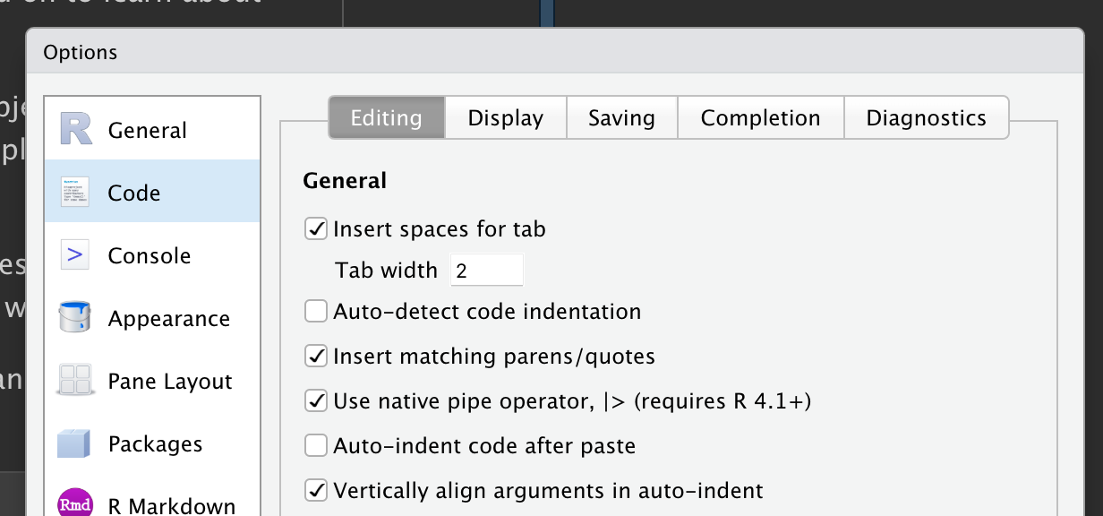
|>,请确保勾选了“使用原生管道运算符”选项。
magrittr
如果你已经使用 tidyverse 一段时间了,你可能熟悉 magrittr 包提供的 %>% 管道。magrittr 包包含在核心 tidyverse 中,所以你可以在加载 tidyverse 时随时使用 %>%:
在简单的情况下,|> 和 %>% 的行为完全相同。那么为什么我们推荐基础管道呢?首先,因为它是 R 基础包的一部分,所以即使你不使用 tidyverse,它也总是可用的。其次,|> 比 %>% 简单得多:在 %>% 于 2014 年发明和 |> 于 2021 年 R 4.1.0 中被包含之间的时间里,我们对管道有了更好的理解。这使得基础实现可以摒弃不常用和不那么重要的功能。
3.5 分组
到目前为止,你已经学习了处理行和列的函数。当你加入处理分组的能力时,dplyr 会变得更加强大。在本节中,我们将重点关注最重要的函数:group_by()、summarize() 以及 slice 系列函数。
3.5.1 group_by()
使用 group_by() 将你的数据集划分为对你的分析有意义的组:
flights |>
    group_by(month)
#> # A tibble: 336,776 × 19
#> # Groups:   month [12]
#>    year month   day dep_time sched_dep_time dep_delay arr_time sched_arr_time
#>   <int> <int> <int>    <int>          <int>     <dbl>    <int>          <int>
#> 1  2013     1     1      517            515         2      830            819
#> 2  2013     1     1      533            529         4      850            830
#> 3  2013     1     1      542            540         2      923            850
#> 4  2013     1     1      544            545        -1     1004           1022
#> 5  2013     1     1      554            600        -6      812            837
#> 6  2013     1     1      554            558        -4      740            728
#> # ℹ 336,770 more rows
#> # ℹ 11 more variables: arr_delay <dbl>, carrier <chr>, flight <int>, …
group_by() 不会改变数据,但如果你仔细看输出,你会注意到输出表明它“按月份分组” (Groups: month [12])。这意味着后续操作现在将“按月”工作。group_by() 将这个分组特性(称为类)添加到数据框中,这改变了应用于该数据的后续动词的行为。
3.5.2 summarize()
最重要的分组操作是摘要 (summary),如果用于计算单个摘要统计量,它会将数据框减少到每个组只有一行。在 dplyr 中,这个操作由 summarize()3 执行,如下例所示,该示例计算了按月份的平均出发延误:
噢!出错了,我们所有的结果都是 NA(发音为“N-A”),这是 R 中表示缺失值的符号。这是因为一些观测到的航班在延误列中有缺失数据,所以当我们计算包含这些值的平均值时,我们得到了 NA 结果。我们将在 Chapter 18 中详细讨论缺失值,但现在,我们将通过将参数 na.rm 设置为 TRUE 来告诉 mean() 函数忽略所有缺失值:
你可以在一次 summarize() 调用中创建任意数量的摘要。你将在接下来的章节中学到各种有用的摘要,但一个非常有用的摘要是 n(),它返回每个组中的行数:
在数据科学中,平均值和计数能让你走得很远!
3.5.3 slice_ 系列函数
有五个方便的函数,允许你在每个组内提取特定的行:
-
df |> slice_head(n = 1)从每个组中取第一行。 -
df |> slice_tail(n = 1)从每个组中取最后一行。 -
df |> slice_min(x, n = 1)取列x值最小的行。 -
df |> slice_max(x, n = 1)取列x值最大的行。 -
df |> slice_sample(n = 1)取一个随机行。
你可以改变 n 来选择多于一行,或者用 prop = 0.1 代替 n = 来选择(例如)每个组中 10% 的行。例如,以下代码找到了在每个目的地到达时延误最严重的航班:
flights |>
    group_by(dest) |>
    slice_max(arr_delay, n = 1) |>
    relocate(dest)
#> # A tibble: 108 × 19
#> # Groups:   dest [105]
#>   dest   year month   day dep_time sched_dep_time dep_delay arr_time
#>   <chr> <int> <int> <int>    <int>          <int>     <dbl>    <int>
#> 1 ABQ    2013     7    22     2145           2007        98      132
#> 2 ACK    2013     7    23     1139            800       219     1250
#> 3 ALB    2013     1    25      123           2000       323      229
#> 4 ANC    2013     8    17     1740           1625        75     2042
#> 5 ATL    2013     7    22     2257            759       898      121
#> 6 AUS    2013     7    10     2056           1505       351     2347
#> # ℹ 102 more rows
#> # ℹ 11 more variables: sched_arr_time <int>, arr_delay <dbl>, …
注意这里有 105 个目的地,但我们得到了 108 行。怎么回事?slice_min() 和 slice_max() 会保留值相同的行,所以 n = 1 意味着给我们所有具有最高值的行。如果你希望每个组只得到一行,你可以设置 with_ties = FALSE。
这类似于用 summarize() 计算最大延误,但你得到的是整个对应的行(如果值相同则有多行),而不是单个摘要统计量。
3.5.4 按多个变量分组
你可以使用多个变量来创建组。例如,我们可以为每个日期创建一个组。
daily <- flights |>
    group_by(year, month, day)
daily
#> # A tibble: 336,776 × 19
#> # Groups:   year, month, day [365]
#>    year month   day dep_time sched_dep_time dep_delay arr_time sched_arr_time
#>   <int> <int> <int>    <int>          <int>     <dbl>    <int>          <int>
#> 1  2013     1     1      517            515         2      830            819
#> 2  2013     1     1      533            529         4      850            830
#> 3  2013     1     1      542            540         2      923            850
#> 4  2013     1     1      544            545        -1     1004           1022
#> 5  2013     1     1      554            600        -6      812            837
#> 6  2013     1     1      554            558        -4      740            728
#> # ℹ 336,770 more rows
#> # ℹ 11 more variables: arr_delay <dbl>, carrier <chr>, flight <int>, …
当你对按多个变量分组的 tibble 进行摘要时,每个摘要都会剥离最后一个分组。事后看来,这不是一个让这个函数工作的很好方式,但在不破坏现有代码的情况下很难改变。为了清楚地说明发生了什么,dplyr 显示了一条消息,告诉你如何改变这种行为:
如果你对这种行为感到满意,你可以明确请求它以抑制该消息:
或者,通过设置不同的值来更改默认行为,例如,"drop" 用于删除所有分组,或 "keep" 用于保留相同的分组。
3.5.5 取消分组
你可能还想在不使用 summarize() 的情况下从数据框中移除分组。你可以使用 ungroup() 来做到这一点。
daily |>
    ungroup()
#> # A tibble: 336,776 × 19
#>    year month   day dep_time sched_dep_time dep_delay arr_time sched_arr_time
#>   <int> <int> <int>    <int>          <int>     <dbl>    <int>          <int>
#> 1  2013     1     1      517            515         2      830            819
#> 2  2013     1     1      533            529         4      850            830
#> 3  2013     1     1      542            540         2      923            850
#> 4  2013     1     1      544            545        -1     1004           1022
#> 5  2013     1     1      554            600        -6      812            837
#> 6  2013     1     1      554            558        -4      740            728
#> # ℹ 336,770 more rows
#> # ℹ 11 more variables: arr_delay <dbl>, carrier <chr>, flight <int>, …
现在让我们看看当你对一个未分组的数据框进行摘要时会发生什么。
你得到了一行,因为 dplyr 将未分组数据框中的所有行都视为属于一个组。
3.5.6 .by
dplyr 1.1.0 包含了一种新的、实验性的、用于按操作分组的语法,即 .by 参数。group_by() 和 ungroup() 不会消失,但你现在也可以使用 .by 参数在单个操作内进行分组:
或者,如果你想按多个变量分组:
.by 适用于所有动词,并且它的优点是,你不需要使用 .groups 参数来抑制分组消息,或者在完成后使用 ungroup()。
我们在本章中没有重点介绍这种语法,因为在我们写书时它还很新。我们想提一下它,因为我们认为它有很大的潜力,很可能会非常流行。你可以在 dplyr 1.1.0 博客文章中了解更多关于它的信息。
3.5.7 练习
哪个航空公司的平均延误最严重?挑战:你能分清是机场不好还是航空公司不好的影响吗?为什么/为什么不?(提示:想想
flights |> group_by(carrier, dest) |> summarize(n()))找出从每个目的地出发时延误最严重的航班。
延误在一天中是如何变化的?用图表来说明你的答案。
如果你向
slice_min()及类似函数提供一个负的n会发生什么?-
假设我们有以下这个小数据框:
- 写下你认为输出会是什么样子,然后检查你是否正确,并描述
group_by()的作用。
df |>
  group_by(y)
b. 写下你认为输出会是什么样子,然后检查你是否正确,并描述 `arrange()` 的作用。另外,评论它与 (a) 部分中的 `group_by()` 有何不同。df |> arrange(y)c. 写下你认为输出会是什么样子,然后检查你是否正确,并描述这个管道的作用。d. 写下你认为输出会是什么样子,然后检查你是否正确,并描述这个管道的作用。然后,评论消息说了什么。- 写下你认为输出会是什么样子,然后检查你是否正确,并描述这个管道的作用。它的输出与 (d) 部分的输出有何不同?
- 写下你认为输出会是什么样子,然后检查你是否正确,并描述每个管道的作用。这两个管道的输出有何不同?
- 写下你认为输出会是什么样子,然后检查你是否正确,并描述
3.6 案例
每当你进行任何聚合操作时,包含一个计数(n())总是一个好主意。这样,你可以确保你不是基于非常少量的数据得出结论。我们将用 Lahman 包中的一些棒球数据来演示这一点。具体来说,我们将比较一个球员击中安打(H)的比例与他们尝试将球打入场内(AB)的次数:
batters <- Lahman::Batting |>
    group_by(playerID) |>
    summarize(
        performance = sum(H, na.rm = TRUE) / sum(AB, na.rm = TRUE),
        n = sum(AB, na.rm = TRUE)
    )
batters
#> # A tibble: 20,730 × 3
#>   playerID  performance     n
#>   <chr>           <dbl> <int>
#> 1 aardsda01      0          4
#> 2 aaronha01      0.305  12364
#> 3 aaronto01      0.229    944
#> 4 aasedo01       0          5
#> 5 abadan01       0.0952    21
#> 6 abadfe01       0.111      9
#> # ℹ 20,724 more rows
当我们绘制击球手的技术水平(用击球率 performance 衡量)与击球机会次数(用打数 n 衡量)的关系图时,你会看到两种模式:
在打数较少的球员中,
performance的变异更大。这个图的形状非常有特点:每当你绘制平均值(或其他摘要统计量)与组大小时,你都会看到随着样本量的增加,变异会减小4。技术水平 (
performance) 和击球机会 (n) 之间存在正相关关系,因为球队希望给他们最好的击球手最多的击球机会。
batters |>
    filter(n > 100) |>
    ggplot(aes(x = n, y = performance)) +
    geom_point(alpha = 1 / 10) +
    geom_smooth(se = FALSE)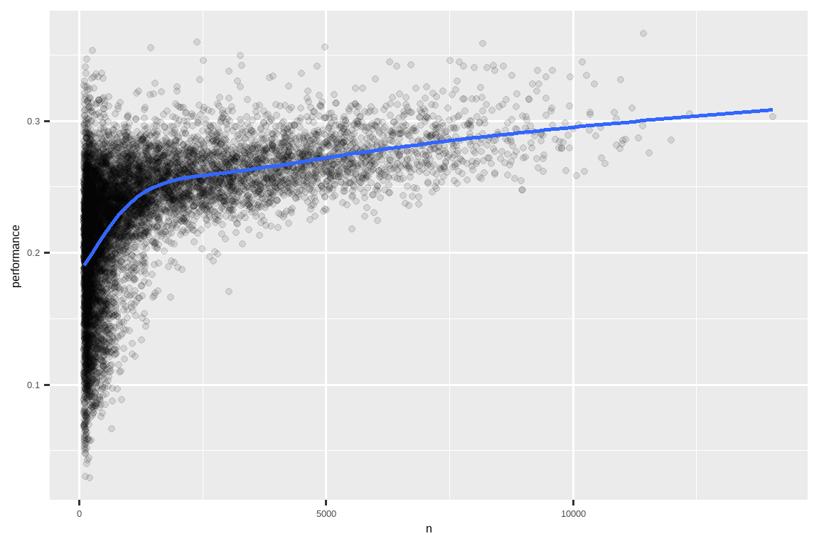
注意 ggplot2 和 dplyr 组合使用的便捷模式。你只需要记住从用于数据处理的 |> 切换到用于向图表添加图层的 +。
这对排名也有重要影响。如果你天真地按 desc(performance) 排序,击球率最高的人显然是那些尝试将球打入场内次数很少且碰巧击中安打的人,他们不一定是最有技术的球员:
你可以在 http://varianceexplained.org/r/empirical_bayes_baseball/ 和 https://www.evanmiller.org/how-not-to-sort-by-average-rating.html 找到对这个问题以及如何克服它的很好解释。
3.7 小结
在本章中,你学习了 dplyr 为处理数据框提供的工具。这些工具大致分为三类:操作行的(如 filter() 和 arrange()),操作列的(如 select() 和 mutate()),以及操作分组的(如 group_by() 和 summarize())。在本章中,我们重点关注了这些“整个数据框”的工具,但你还没有学到太多关于可以对单个变量做什么的知识。我们将在本书的“转换”部分回到这个问题,其中每一章都为特定类型的变量提供工具。
在下一章中,我们将转回工作流程,讨论代码风格的重要性以及保持代码良好组织,以便你和他人都能轻松阅读和理解。