4  Density

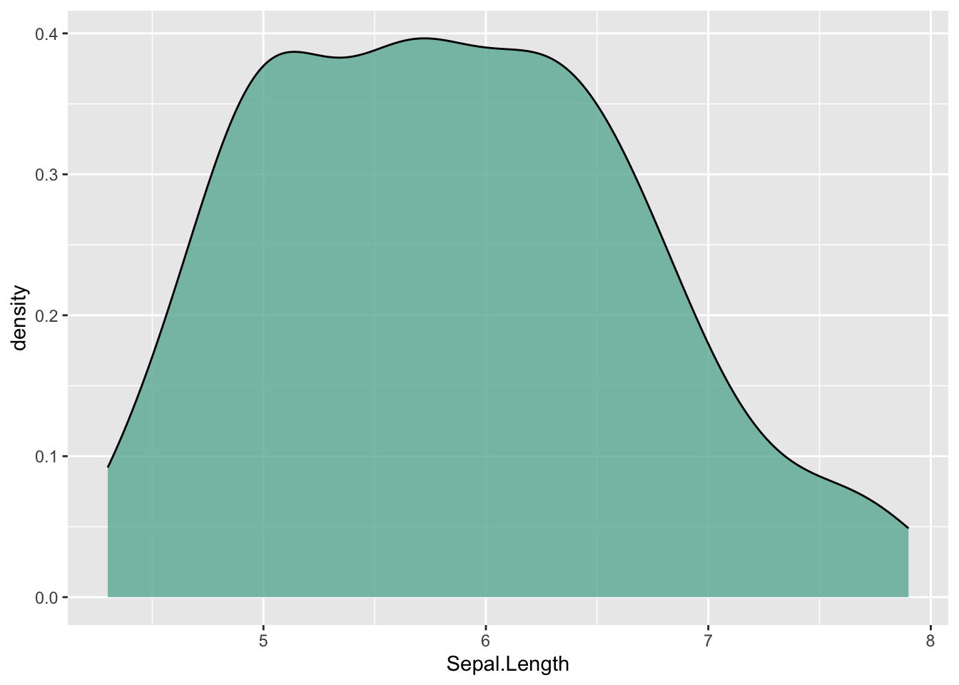
核密度曲线图其实是一个平滑的直方图，曲线下面积是1。

通过geom_density()函数可以绘制核密度曲线图。

4.1 单组

library(tidyverse)

ggplot(iris, aes(x = Sepal.Length)) + 
  geom_density(fill="#69b3a2", alpha=0.8) # 可选主题 theme_ipsum()

基本的geom_density

4.2 多组

4.2.1 镜像

镜像密度曲线图见 Section 2.1.2

4.2.2 分组和分面

ggplot(iris, aes(x = Sepal.Length, fill = Species), ) + 
  geom_density(alpha=0.8)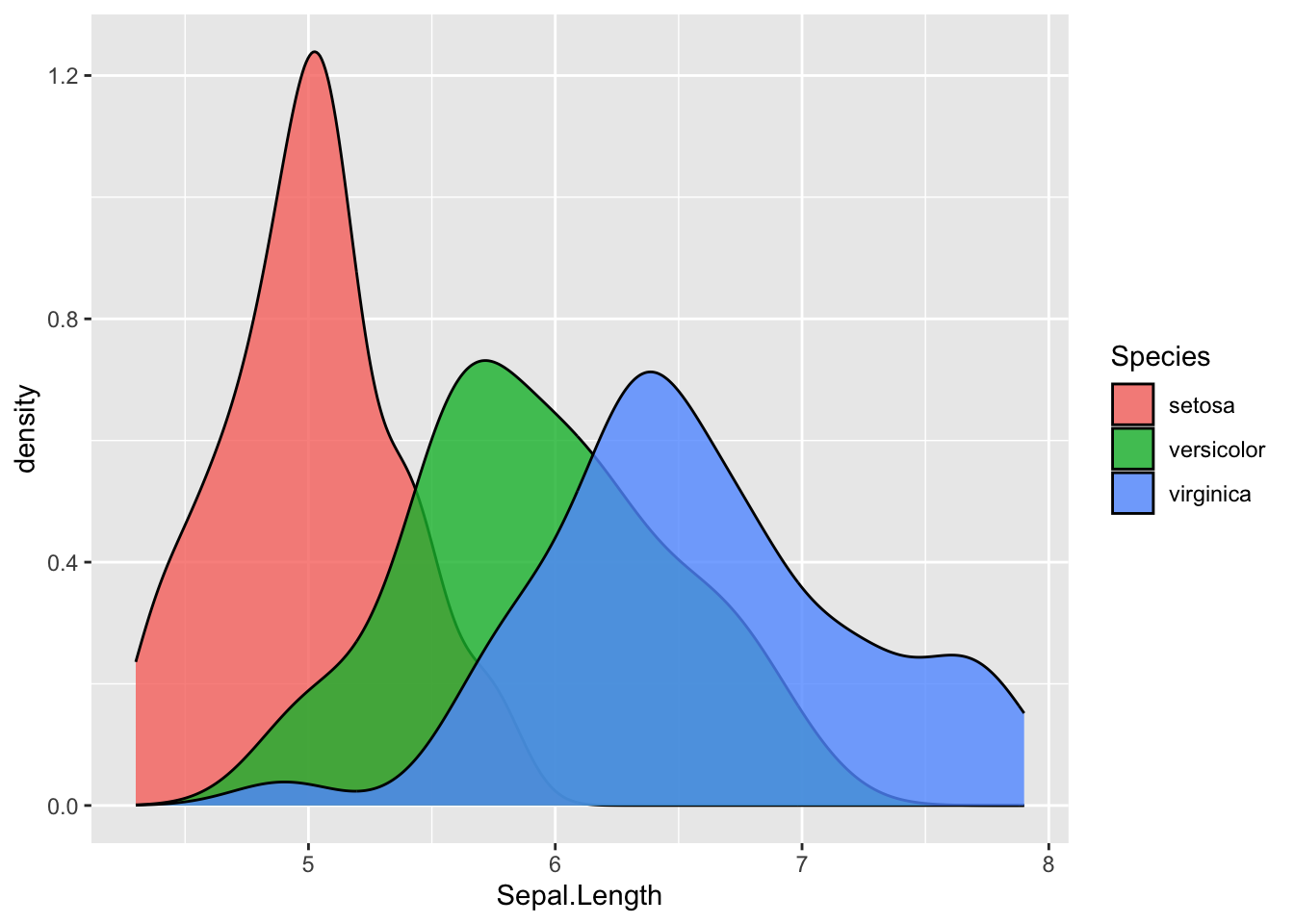

分组

ggplot(iris, aes(x = Sepal.Length, fill = Species)) + 
  geom_density(alpha=0.8) + 
  facet_wrap(~ Species) + 
  theme(legend.position = "none")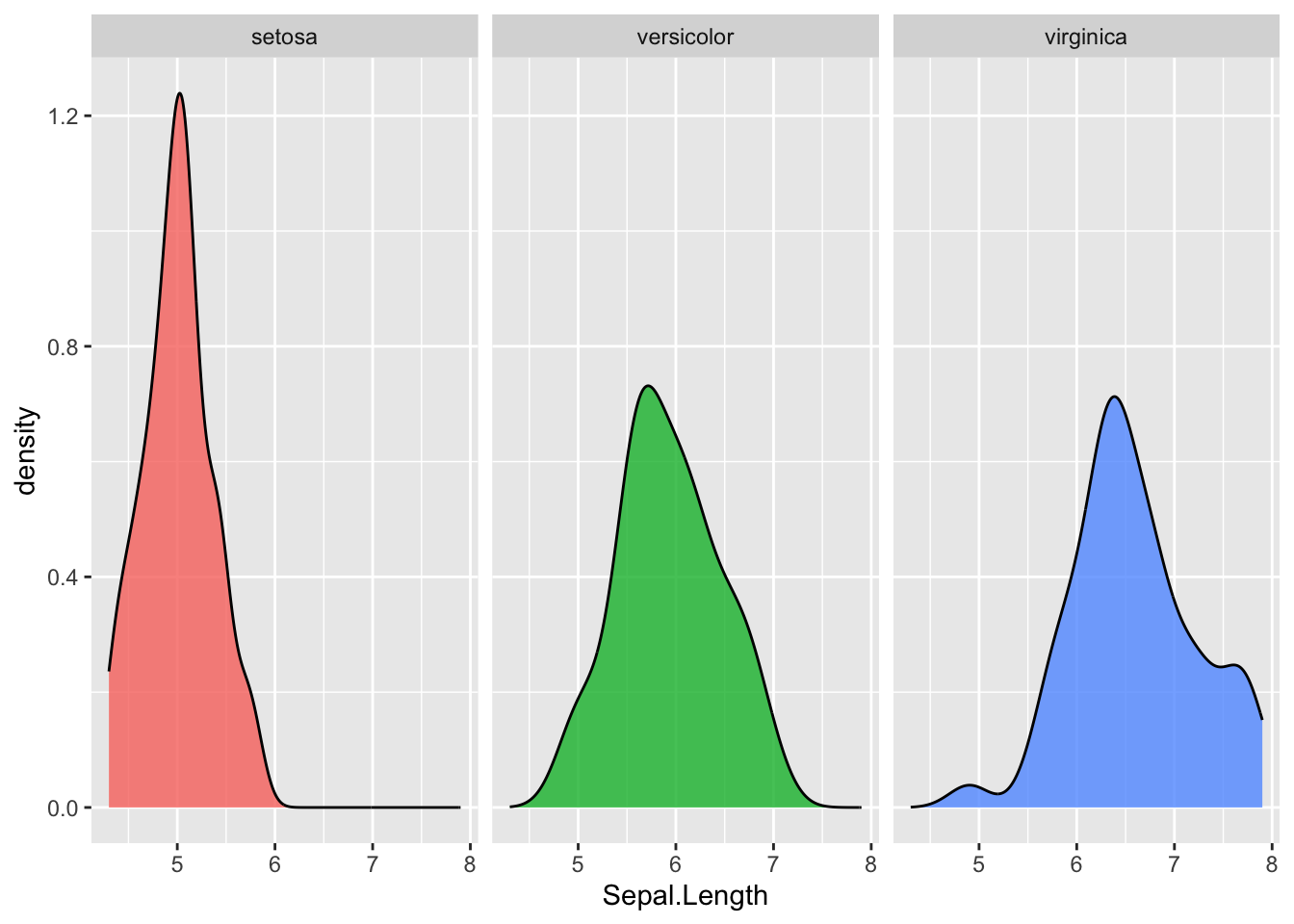

分面

4.2.3 山脊图

分面不如山脊图好看，见 Chapter 5

4.2.4 堆叠

通过position=“fill”绘制堆叠密度图，可以看到每个组的比例

library(hrbrthemes) # theme_ipsum
ggplot(data=diamonds, aes(x=price, group=cut, fill=cut)) +
    geom_density(adjust=1.5, position="fill") +
    theme_ipsum()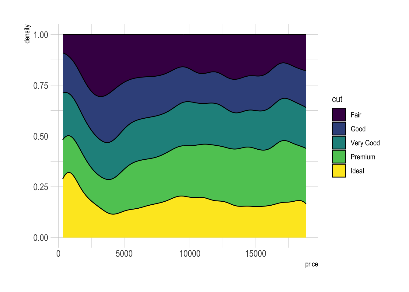

堆叠密度图

4.3 注释/标签

还可以使用annot数据框来添加注释，下面的例子中，我们在鸢尾花的密度曲线上添加了每个物种的名称注释。

4.3.1 geom_text

annot <- data.frame(
  Species = c("setosa", "versicolor", "virginica"),
  x = c(5.2, 5.5, 6.4),
  y = c(1.2, 0.8, 0.8)
)

ggplot(iris, aes(x = Sepal.Length, fill = Species)) + 
  geom_density(alpha=0.8)  +
  geom_text(data=annot, aes(x=x, y=y, label=Species, color=Species), hjust=0, size=4.5) +
  theme_ipsum() + # 适合印刷的主题
  theme(legend.position = "none")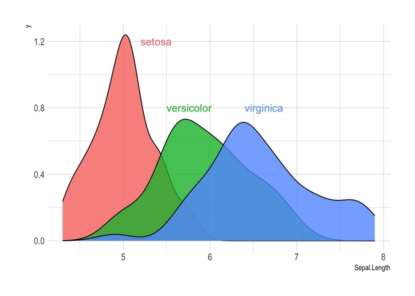 

带注释的密度曲线图

4.3.2 textdensity

library(geomtextpath)
library(hrbrthemes)

ggplot(iris, aes(x = Sepal.Length, color = Species, label = Species)) +
  geom_textdensity() + 
  theme_bw() + 
  theme(legend.position = "none")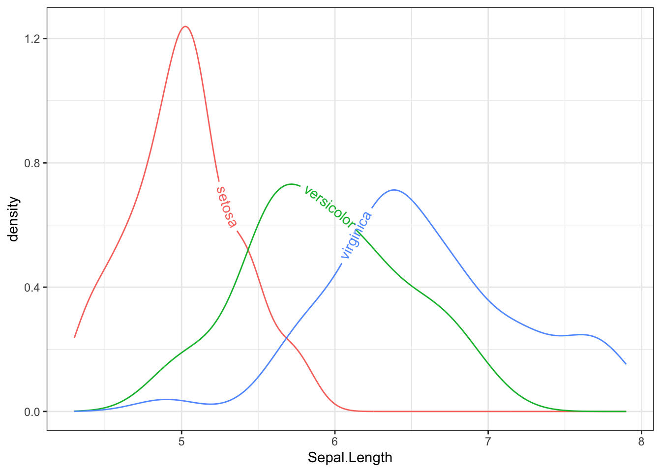

geomtextpath 更方便添加标签,但是不能带fill颜色

library(geomtextpath)
library(hrbrthemes)

ggplot(iris, aes(x = Sepal.Length, color = Species, label = Species)) +
  geom_textdensity(vjust = -0.4, hjust = "ymid") + # hjust = "ymid" 调整标签位置
  theme_bw() + 
  theme(legend.position = "none")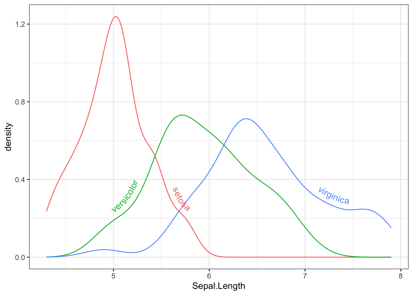

geomtextpath 调整标签位置

text参数:

• size: 文本大小
• fontface: 字体样式
• vjust: 垂直调整
• hjust: 水平调整

r-graph-gallery 还有一些示例: geomtextpath

4.4 边缘图

见 Section 3.3.9